Computer Vision Research & Engineering

Real-World Vision
Systems That Deploy.

Lightweight deep learning for semantic segmentation, object detection, and edge AI across intelligent transportation, UAV analytics, medical imaging, industrial inspection, and aviation safety.

11+
Years Research Experience
29+
Research Contributions
15+
Vision Models Developed
Multi
Application Domains
Inference Demos

Model Inference in Action.

Selected Projects

Published Architectures.

Research-driven lightweight architectures designed for deployment-aware computer vision systems where accuracy, efficiency, and real-world constraints matter.

Applications

Vision AI Across
Real-World Domains.

Some of the application domains where deployment-aware computer vision systems can support real-world analysis, monitoring, and automation.

Computer Vision Research & Engineering

Lightweight Vision Systems
From Architecture Design to Inference.

Semantic Segmentation

Lightweight encoder-decoder systems for pixel-level analysis across medical imaging, infrastructure monitoring, aerial analytics, and vision-driven applications.

LiteFusionNet DFF-UNet

Object Detection

Efficient detection systems for small objects, visual monitoring, and constrained computer vision applications.

VDXNet LiteFODNet

Lightweight Architecture

Parameter-efficient architectures balancing accuracy, latency, computational cost, and memory constraints for efficient vision systems.

Parameter Efficiency Low GFLOPs

Inference Optimization

TensorRT optimization, ONNX deployment workflows, FP32/FP16 benchmarking, and hardware-aware performance evaluation for embedded vision systems.

TensorRT Jetson
Blog

Technical Articles
Insights, Engineering, & Experiments.

Debugging & Failure Analysis

Why Your Segmentation Model Predicts Only Background (And How to Fix It)

Root cause analysis of foreground collapse under cross-entropy on imbalanced datasets. CVC-ClinicDB experiment over 100 epochs.

Practical Guide

How to Train an Object Detection Model on a Custom Dataset (What Tutorials Don't Tell You)

The decisions tutorials skip, dataset format, model scale, evaluation methodology. YOLOv12 on VisDrone.

Architecture

U-Net Explained Clearly (With a Practical Training Example)

Encoder, skip connections, and decoder from first principles. CVC-ClinicDB training results across 100 epochs.

Debugging & Failure Analysis

Common Mistakes in Object Detection Training That Kill Performance

Wrong annotations, bad augmentation, poor evaluation, and overfitting, each with symptom patterns and fixes.

Read All Articles
Books

Beginner to Advanced.
Two Tracks.

Semantic Segmentation Track
A Step-by-Step Guide for BeginnersBeginner
Training Models on Real-World DataIntermediate
Advanced Architecture Design and ExperimentsAdvanced
Object Detection Track
A Step-by-Step Guide for BeginnersBeginner
Training Models on Real-World DatasetsIntermediate
Advanced Architecture Design and ExperimentsAdvanced
Browse Books

Discuss a Computer Vision Project

Whether you are improving a lightweight architecture, optimizing deployment performance, designing a segmentation system, or exploring a computer vision solution. Occulins provides focused technical consultation and development support.

Services

Computer Vision Research & Engineering.

Lightweight architecture development, deployment-focused engineering, and technical consultation for real-world computer vision systems.

Computer Vision Research & Engineering

Core Services.

Semantic Segmentation Systems

Precise Pixel-Level Analysis

Custom segmentation systems for research and applied computer vision tasks requiring accurate region, boundary, or object-level understanding.

  • Efficient encoder-decoder architectures
  • Context-aware feature learning
  • Lightweight segmentation pipelines
  • Deployment-aware experimentation
Object Detection Systems

Lightweight Detection for Real Environments

Efficient detection systems for visual recognition tasks where accuracy, speed, and computational cost must be balanced.

  • Small-object and multi-scale detection
  • YOLO-family customization
  • Backbone, neck, and head design
  • Deployment-aware evaluation
Lightweight Model Design

Architecture Under Computational Constraints

Design and refinement of compact deep learning architectures for scenarios where parameter count, GFLOPs, latency, and memory matter.

  • Parameter-efficient modules
  • Multi-scale feature fusion
  • Attention and context modules
  • Accuracy-efficiency trade-off analysis
Deployment Support

Model Optimization & Inference Acceleration

Support for moving trained vision models toward efficient runtime behavior through export, optimization, and deployment-aware testing.

  • ONNX export support
  • TensorRT optimization
  • Inference acceleration & latency analysis
  • Runtime benchmarking and deployment review
Technical AI Consultation
Focused Technical Sessions

Technical AI Consultation

Scheduled, topic-focused sessions for researchers, engineers, and organizations working on computer vision systems.

  • Architecture selection & review
  • Debugging training issues
  • Deployment planning & optimization
  • Evaluation methodology
  • Experimentation strategy
Basic1-Hour Session

Targeted discussion around a specific challenge, deployment issue, architecture decision, or experimental problem.

Standard2-Hour Session

Extended technical review covering model design, debugging, deployment considerations, or experimental analysis.

Consultation scope and engagement structure are determined based on project requirements.
Start a Project Discussion
Books

Detection & Segmentation.
Structured Learning Tracks.

Choose a structured track for object detection or semantic segmentation from foundations to real-world experiments and architecture design.

Semantic Segmentation Track

Semantic Segmentation Track

Three books covering segmentation foundations, training workflows, debugging, architecture design, and experiment analysis.

Explore Track
Object Detection Track

Object Detection Track

Three books covering YOLO workflows, dataset preparation, training, evaluation, architecture design, and deployment-oriented experimentation.

Explore Track
Books

Semantic Segmentation
Book Track.

A three-book path covering segmentation foundations, real-world training, debugging, architecture design, and experiment analysis.

Segmentation Book 1 preview
Beginner
Practical Semantic Segmentation with Deep Learning
A Step-by-Step Guide for Beginners
By the end of this book, you'll able to:
  • Understand the fundamentals of semantic segmentation and pixel-wise prediction
  • Prepare segmentation datasets, masks, and training pipelines correctly
  • Train and evaluate U-Net models using standard segmentation metrics
  • Interpret prediction errors and common segmentation failure cases
  • Build a complete semantic segmentation project from dataset to inference
PDF • 46 pages • Companion Resources Included
Preview
Segmentation Book 2 preview
Intermediate
Practical Semantic Segmentation with Deep Learning
Training Models on Real-World Data
By the end of this book, you'll able to:
  • Analyze real-world segmentation problems before model development
  • Build reliable training pipelines for domain-specific datasets
  • Diagnose and resolve common training and evaluation issues
  • Improve segmentation performance through practical experimentation
  • Develop segmentation workflows suitable for real-world applications
PDF • 50 pages • Companion Resources Included
Preview
Segmentation Book 3 preview
Advanced
Practical Semantic Segmentation with Deep Learning
Advanced Architecture Design and Experiments
By the end of this book, you'll able to:
  • Analyze modern segmentation architectures and their design principles
  • Design efficient feature extraction and feature fusion modules
  • Evaluate architectural improvements through systematic experimentation
  • Balance accuracy, efficiency, and computational complexity
  • Develop research-oriented segmentation models for real-world deployment
PDF • 54 pages • Companion Resources Included
Preview

← Back to Books

Books

Object Detection
Book Track.

A three-book path covering YOLO foundations, custom dataset training, evaluation workflows, architecture design, and deployment-oriented experimentation.

Detection Book 1 preview
Beginner
Practical Object Detection with YOLO
A Step-by-Step Guide for Beginners
By the end of this book, you'll able to:
  • Understand modern object detection and the YOLO workflow
  • Prepare datasets and annotations for reliable model training
  • Train and evaluate YOLO models using standard detection metrics
  • Interpret prediction errors and improve detection performance
  • Build a complete object detection project from dataset to inference
PDF • 44 pages • Companion Resources Included
Preview
Detection Book 2 preview
Intermediate
Practical Object Detection with YOLO
Training Models on Real-World Datasets
By the end of this book, you'll able to:
  • Analyze real-world detection problems and domain-specific datasets
  • Build reliable training pipelines for practical detection tasks
  • Adapt pretrained models to new domains through transfer learning
  • Improve detection performance for challenging real-world scenarios
  • Develop end-to-end detection workflows for deployment
PDF • 59 pages • Companion Resources Included
Preview
Detection Book 3 preview
Advanced
Practical Object Detection with YOLO
Advanced Detection Architecture Design and Experiments
By the end of this book, you'll able to:
  • Analyze the design principles of modern object detectors
  • Design lightweight modules for efficient feature extraction and fusion
  • Evaluate architectural improvements through rigorous experimentation
  • Balance detection accuracy with computational efficiency
  • evelop research-oriented detection models for practical deployment
PDF • 76 pages • Companion Resources Included
Preview

← Back to Books

Blog

Technical Articles
Insights, Engineering, & Experiments.

Research-driven articles on semantic segmentation, object detection, architecture design, and deployment-aware engineering.

BCE vs BCE+Dice sensitivity training curve
Debugging & Failure Analysis

Why Your Segmentation Model Predicts Only Background

Root-cause analysis of foreground collapse, class imbalance, loss selection, and prediction diagnostics in segmentation systems.

Practical Guide

How to Train an Object Detection Model on a Custom Dataset

Practical decisions behind dataset setup, configuration, evaluation, and common failure points in detection experiments.

U-Net architecture diagram
Architecture Explained

U-Net Explained Clearly (With a Practical Training Example)

Why U-Net is shaped the way it is, how skip connections solve the spatial precision problem, and what training on CVC-ClinicDB actually looks like across 100 epochs.

Healthy vs overfitting loss curves
Debugging & Failure Analysis

Common Mistakes in Object Detection Training That Kill Performance

Four training mistakes that are invisible in your loss curves — wrong annotations, harmful augmentation, misleading evaluation, and hidden overfitting with specific symptoms and fixes for each.

Selected Projects

Selected Projects.

A curated portfolio of computer vision research and engineering projects built from peer-reviewed work, lightweight deep learning, and deployment-aware vision systems.

DFF-UNet Architecture
IEEE Trans. Instrumentation & MeasurementVol. 74 · 2025Segmentation
DFF-UNet

DFF-UNet: A Lightweight Deep Feature Fusion U-Net Model for Skin Lesion Segmentation

RFRE encoder with adaptive 3×3 and 1×1 convolutions, PDCP bridge with parallel dilated convolutions at rates (1,3,5), and BSFD decoder using bottleneck blocks and depthwise separable convolutions.

mIoU 0.7926Dice 0.88430.190M params0.109 GFLOPs1.30ms
97.55% fewer parameters and 99.20% fewer GFLOPs than U-Net. Best on ISIC2018. Validated on 4 public datasets.
LiteFusionNet Architecture
Advanced Engineering InformaticsVol. 65 · 2025Segmentation
LiteFusionNet

Advancing Road Safety: A Lightweight Feature Fusion Model for Robust Road Crack Segmentation

Lightweight encoder with residual blocks, DGA, and DVM modules; EASPP bridge for multi-scale crack feature extraction; Dual-Level Decoder with 3×3 convolutions and channel attention.

Dice 0.7828mIoU 0.64310.493M params0.397 GFLOPs
Outperforms SegNet (29.44M params) with 98.3% fewer parameters. Best Dice on Crack500, DeepCrack, and RCD.
VDXNet Architecture
IEEE Geoscience & Remote Sensing LettersVol. 22 · 2025Detection
VDXNet

VDXNet: A Novel Lightweight Deep Learning Model for Vehicle Detection With Aerial Images

RxDF module with asymmetric depthwise separable convolutions replaces C3K2; LiteFPP with selective pooling at 5×5 and 9×9 replaces SPPF; CRDown replaces Conv at P5.

mAP 96.3% (UCAS-AOD)mAP 98.9% (UAVDT)1.608M params539 FPS
37.72% fewer parameters than YOLO11n while improving mAP by 0.52%. Best across all four aerial datasets.
LiteFODNet Architecture
Intelligent Data Analysis · SAGE/IOS2025Detection
LiteFODNet

LiteFODNet: A Lightweight Deep Learning Model for Intelligent Detection of Small Objects in Runway Surveillance Data

CMSP with parallel atrous convolutions replaces SPPF; SCR replaces Conv at P5; FFM for channel-wise calibration; SPA with decoupled height/width attention for small object localization.

mAP@50-95 0.6812.515M params1.3ms
+0.89% mAP vs YOLOv8n with −16.4% parameters and −27.8% inference time.
CigDet · SURRONE Architecture
Expert Systems with Applications · ElsevierVol. 267 · 2025Review & Dataset
CigDet · SURRONE

Deep Learning-Based Smoker Classification and Detection: An Overview and Evaluation

Comprehensive survey introducing CigDet — a novel annotated dataset for cigarette localization (open-source, Mendeley Data). Benchmarks YOLOv1 through YOLO11. Proposes the SURRONE drone-based outdoor surveillance framework.

YOLOv9 mAP 83.50%YOLO11 mAP 81.50%11 YOLO variants557 annotated images
First open-source annotated dataset for cigarette localization. First benchmark of all YOLO variants (v1–v11).
Discuss Computer Vision Work
Resources

Technical Resources.

Protected book companion files, blog code utilities, and curated engineering resources for computer vision workflows.

Book companion resources are organized by track. Resources are provided via post-purchase email.

Semantic Segmentation Track

Companion files for the semantic segmentation book series, loss functions, metric helpers, mask utilities, U-Net references, architecture modules, and experiment support scripts.

Book Resources

Object Detection Track

Companion files for the object detection book series, dataset YAML templates, annotation checks, prediction helpers, evaluation utilities, ONNX export examples, and configuration references.

Book Resources

Companion resources accompanying published Occulins articles, including selected implementations, utilities, configurations, and supporting materials for practical experimentation and workflow understanding.

Blog 1 Companion Resources

Supporting resources for segmentation debugging and foreground-collapse analysis, including U-Net implementation, loss functions, metric utilities, visualization helpers, foreground diagnostics, and experiment configuration.

Companion Assets

Blog 2 Companion Resources

Supporting resources for custom YOLO training workflows on VisDrone, including dataset validation, YAML configuration, training utilities, prediction workflows, and evaluation guidance.

Companion Assets

Blog 3 Companion Resources

Supporting resources for the U-Net architecture explanation, including model implementation, DoubleConv block, architecture configuration, skip-connection reference, and selected plotting utilities.

Companion Assets

Blog 4 Companion Resources

Supporting resources for object detection failure analysis, including missing-label checks, YAML split verification, mAP comparison logic, overfitting diagnostics, and evaluation sanity checks.

Companion Assets

Curated engineering resources for computer vision research, deep learning experimentation, edge AI deployment, robotics, UAV systems, and applied AI workflows.

Some links on this page may be affiliate links in the future. Occulins may earn a small commission at no additional cost to you. Recommendations are selected based on technical relevance, practical workflow value, and suitability for computer vision or edge AI experimentation.

Compute & Training Hardware

Resource Best For Technical Notes Status
RTX 4090/5090 24GB Heavy segmentation and detection training Higher VRAM capacity supports larger input resolutions, heavier architectures, and larger batch sizes for deep learning experiments. Coming Soon
RTX 4080/5080 16GB Mid-to-high range experimentation Useful for moderate segmentation and detection workloads with lower cost and power requirements than flagship GPUs. Coming Soon
RTX 4070/5070 16GB Lightweight to moderate AI research Suitable for lightweight computer vision experimentation, architecture debugging, and deployment-focused model development. Coming Soon
NVMe SSD 2TB Dataset storage and fast experiment loading Useful when working with image datasets, checkpoints, logs, and repeated training runs. Coming Soon

Edge AI & Deployment Devices

Resource Best For Technical Notes Status
Jetson Orin Nano TensorRT FP16 deployment experiments Useful for lightweight object detection and segmentation inference testing on embedded AI hardware. Coming Soon
Jetson Orin NX Higher-performance edge AI deployment Suitable for heavier real-time computer vision workloads where embedded inference performance matters. Coming Soon
Raspberry Pi AI Kit Low-power AI prototyping Useful for small embedded AI demonstrations and lightweight inference experiments. Coming Soon

Vision Sensors, Robotics & UAV Hardware

Resource Best For Technical Notes Status
USB / RGB Camera Module Real-time detection and segmentation demos Useful for prototyping image acquisition pipelines and live computer vision experiments. Coming Soon
Thermal Camera Module Multimodal and environmental monitoring Relevant for RGB-thermal object detection, fire monitoring, surveillance, and low-light perception workflows. Coming Soon
AI Robotic Car Kit Autonomous driving demonstrations Useful for lane detection, obstacle detection, small-scale perception, and robotics vision experiments. Coming Soon
UAV / Drone Platform Aerial analytics and remote sensing experiments Useful for UAV-based crack detection, aerial object detection, forest monitoring, and environmental inspection workflows. Coming Soon

Books & Technical References

Resource Best For Technical Notes Status
Deep Learning Reference Book Foundational understanding Useful for building stronger intuition around neural networks, optimization, and representation learning. Coming Soon
Computer Vision Reference Book Computer vision fundamentals Useful for understanding classical and modern vision concepts before moving into applied deep learning systems. Coming Soon
PyTorch Reference Book Implementation and experimentation Useful for researchers and engineers implementing models, training loops, debugging, and deployment pipelines. Coming Soon

Resource Policy

Protected book resources may include selected model files, configuration files, modules, architecture references, and companion assets. Full proprietary repositories, commercial training frameworks, and complete production pipelines are not publicly distributed unless explicitly stated otherwise. Blog companion code may be released separately as open source where applicable.

Recommendations and external resource references are included for educational, research, and workflow guidance purposes. Some links may be affiliate links.

Affiliate Disclosure

About

About Occulins.

Computer vision research and engineering for deployment-aware systems built for real-world constraints.

Occulins is a computer vision research and engineering lab specializing in lightweight deep learning systems for semantic segmentation, object detection, and deployment-aware vision engineering.

Our work focuses on designing efficient computer vision architectures that balance accuracy, inference speed, parameter efficiency, and deployment constraints across medical imaging, aerial analytics, intelligent transportation, infrastructure monitoring, industrial inspection, aviation safety, and edge AI systems.

Built on years of research experience in deep learning and computer vision, Occulins focuses on translating research into practical engineering workflows. Every architecture is developed with practical constraints in mind, including latency, memory usage, computational efficiency, embedded inference, and real-world deployment requirements.

Occulins is evolving toward a full computer vision research and engineering lab focused on intelligent vision systems, scalable AI infrastructure, and practical computer vision technologies for industry and research-driven applications.

We collaborate on computer vision problems requiring both research depth and practical deployment awareness across constrained and real-world environments.

Lightweight Architecture Design

Parameter-efficient architectures designed for balanced accuracy, computational efficiency, reduced memory footprint, and deployment-aware inference.

Semantic Segmentation

Encoder-decoder systems for pixel-level scene understanding across medical, infrastructure, aerial, and industrial imaging domains.

Object Detection

Real-time detection systems for visual monitoring, small object analysis, dense scenes, and deployment-constrained computer vision applications.

Inference Optimization & Deployment

Model optimization, deployment workflows, TensorRT acceleration, ONNX export, FP32/FP16 benchmarking, and hardware-aware performance evaluation.

Computer Vision Research & Engineering

Computer vision research, architecture design, and system development for domain-specific applications across research and industry.

Contact

Start a Project Discussion.

Focused technical consultation and development support for applied computer vision systems.

Get in Touch

Occulins works with researchers, startups, and technical teams on lightweight computer vision systems, model optimization, and deployment-aware AI solutions.

ResponseWithin 48 hours
Relevant inquiries are typically answered within 48 hours. Project scope and engagement structure are discussed before any work begins.
Project Detail

LiteFusionNet.

A lightweight road-crack segmentation architecture designed for efficient infrastructure monitoring under strict model-size and computation constraints.

Semantic Segmentation

Architecture Overview

LiteFusionNet is designed for road-crack segmentation where thin structures, cluttered road textures, and deployment constraints make dense prediction difficult. The architecture keeps a compact encoder–decoder structure while strengthening feature extraction through residual blocks, dilated gated attention, and dual vision mamba components. Its EASPP bridge captures crack-related context across multiple receptive fields, while the Dual-Level Decoder combines low-level spatial details with high-level contextual cues for sharper pixel-level localization. The result is an efficient segmentation model intended for infrastructure monitoring scenarios where accuracy, parameter count, and GFLOPs must be balanced rather than optimized in isolation.

0.493M parameters0.397 GFLOPsEASPP multi-scale bridgeDual-Level Decoder

Architecture Diagram

litefusionnet architecture diagram
Project Detail

DFF-UNet.

A compact skin-lesion segmentation model with RFRE encoder, PDCP bridge, and BSFD decoder for dermoscopic image analysis.

Medical Image Segmentation

Architecture Overview

DFF-UNet targets skin-lesion segmentation with a compact U-shaped design that focuses on boundary precision and computational efficiency. The RFRE encoder refines feature extraction through residual connections and adaptive convolutional processing, while the PDCP bridge captures contextual lesion patterns using parallel dilated convolutions. The BSFD decoder then fuses semantic and spatial information through bottleneck-based skip fusion, allowing the model to preserve important lesion details without increasing complexity. This makes the architecture suitable for dermoscopic image analysis where precise segmentation and lightweight deployment are both important.

0.190M parameters0.109 GFLOPsRFRE encoderPDCP + BSFD design

Architecture Diagram

dffunet architecture diagram
Project Detail

VDXNet.

A real-time aerial vehicle detection architecture using RxDF, LiteFPP, and CRDown components for UAV and aerial imagery.

Aerial Object Detection

Architecture Overview

VDXNet is a lightweight aerial vehicle detection model built for intelligent transportation and remote-sensing scenarios. Its design replaces heavier feature aggregation components with RxDF modules that combine spatial and depthwise information efficiently. LiteFPP supports multiscale contextual representation, while CRDown reduces spatial dimensions with lower computational cost. This architecture is shaped around the practical difficulty of detecting small vehicles with different orientations and background clutter, while keeping the model efficient enough for real-time aerial monitoring workflows.

1.608M parameters5.9 GFLOPsRxDF feature fusionLiteFPP + CRDown

Architecture Diagram

vdxnet architecture diagram
Project Detail

LiteFODNet.

A lightweight FOD detection model for airport runway safety and small-object detection in cluttered visual conditions.

Foreign Object Debris Detection

Architecture Overview

LiteFODNet is designed for small foreign object debris detection in runway surveillance imagery, where targets are visually diverse, sparse, and often difficult to separate from complex backgrounds. The architecture introduces CMSP for compact multiscale context, SCR for efficient downsampling, FFM for channel-level feature calibration, and SPA for spatial attention along separate axes. Together, these modules guide the detector toward small, ambiguous objects while controlling computational burden. The model is positioned for aviation safety monitoring where real-time inference and reliable small-object localization are critical.

Small-object detectionCMSP multiscale poolingSCR downsamplingFFM + SPA attention

Architecture Diagram

litefodnet architecture diagram
Project Detail

CigDet / SURRONE.

A smoker/cigarette detection dataset and surveillance-oriented research framework benchmarking YOLO variants for environmental and safety monitoring.

Dataset and Review Framework

Architecture Overview

CigDet / SURRONE represents the environmental and safety monitoring direction of Occulins. The work combines dataset development, YOLO-based benchmarking, and a drone-oriented conceptual framework for cigarette and smoker detection. Instead of focusing only on model accuracy, the project highlights the practical deployment challenges of monitoring open environments, including small target localization, scene variability, and operational constraints. It provides a foundation for future lightweight detection systems in public-health, surveillance, and environmental monitoring scenarios.

CigDet datasetYOLO benchmarkingDrone-based frameworkEnvironmental monitoring

Architecture Diagram

surrone architecture diagram
Application Domain

Infrastructure Monitoring.

Automated visual analysis of civil infrastructure using lightweight computer vision, enabling detection and segmentation of surface conditions, structural elements, and anomalies at scale.

Infrastructure AI
Computer vision for infrastructure monitoring.

Infrastructure assets degrade continuously through weather, load cycles, and material fatigue. Lightweight vision models enable automated detection of road cracks, bridge spalling, corrosion, and structural deformation from standard camera and drone imagery providing consistent coverage across large asset portfolios where manual inspection is impractical at scale. Models are designed to operate across varied surface types and imaging conditions, supporting deployment in both fixed-camera monitoring systems and UAV-based inspection workflows.

Surface analysisStructural inspectionDefect localizationAutomated monitoring
Infrastructure Monitoring segmentation output
Infrastructure Monitoring object detection output

Object Detection

Detection and localization of surface defects, damage types, and structural anomalies for infrastructure health assessment and maintenance prioritization.

Infrastructure Monitoring semantic segmentation result

Semantic Segmentation

Pixel-level segmentation of road surfaces, bridge decks, and structural facades, enabling precise crack boundary delineation, spalling localization, and defect extent quantification for maintenance prioritization.

Benefits

Why Computer Vision Matters
in Infrastructure Monitoring.

01 — Detect defects before they become failures

Automated crack and spalling detection identifies surface deterioration weeks or months before it reaches the threshold requiring emergency repair reducing the likelihood of costly structural failures and unplanned road closures.

02 — Cut field survey time significantly

Image-based inspection of roads, bridges, and facades processes in seconds what takes field teams hours on-site. Coverage that previously required days of manual survey can be completed from drone or vehicle-mounted camera footage in a fraction of the time.

03 — Scale across entire road and asset networks

Lightweight models handle thousands of images per day without proportional increases in cost or staffing, making city-scale crack mapping and bridge monitoring operationally feasible for the first time.

04 — Reach assets that are unsafe to inspect manually

Elevated structures, active carriageways, and confined spaces that carry significant risk for inspection personnel can be assessed remotely using UAV-deployed vision systems with no access constraints.

← Back to Home
Application Domain

Medical Imaging.

Lightweight AI for clinical image analysis, enabling automated detection and segmentation of regions of interest across a range of medical imaging modalities.

Medical AI
Computer vision for medical imaging.

Medical image analysis requires high sensitivity to subtle boundaries and strong generalization across patient populations and imaging conditions. Lightweight architectures designed for clinical deployment provide lesion detection, organ segmentation, and pathology localization across dermatology, histology, and radiology imaging, operating without GPU-heavy infrastructure. Models are built to generalise across patient populations and imaging protocols, supporting integration into clinical review workflows without requiring specialized hardware.

Clinical image analysisRegion of interest detectionDiagnostic supportMulti-modality analysis
Medical Imaging segmentation output
Medical imaging object detection output

Object Detection

Detection and localization of cellular structures, clinical regions of interest, and pathological markers within medical image analysis workflows.

Medical Imaging semantic segmentation result

Semantic Segmentation

Pixel-level delineation of lesion boundaries, organ contours, and pathological regions, supporting precise area measurement, clinical grading, and multi-dataset generalization across imaging modalities.

Benefits

Why Computer Vision Matters
in Medical Imaging.

01 — Reduce variability in clinical image assessment

Automated segmentation and detection provide a consistent baseline across clinicians, imaging sessions, and patient cohorts, reducing the inter-observer disagreement that affects manual region-of-interest identification in dermoscopy, pathology, and radiology.

02 — Quantify lesion boundaries with pixel precision

Segmentation models delineate lesion margins at the pixel level, enabling objective area measurement and boundary characterization that supports clinical grading, treatment response tracking, and longitudinal comparison across patient visits.

03 — Deploy without specialist infrastructure

Sub-megaparam architectures designed for efficiency run on standard clinical workstation hardware without dedicated GPU infrastructure, making AI-assisted image analysis accessible outside large academic medical centers.

← Back to Home
Application Domain

UAV & Aerial Analytics.

Real-time detection and segmentation for UAV platforms, satellite imagery, and aerial imaging systems, enabling automated analysis of scenes, objects, and land cover from elevated viewpoints.

Aerial Vision
Computer vision for aerial analytics.

Aerial imaging introduces unique challenges, small object size, altitude-dependent scale variation, dense scene clutter, and the need for onboard real-time inference under tight power and compute constraints. Lightweight architectures address vehicle detection in satellite imagery, foreign object localization on airport runways, and dense scene segmentation from drone platforms, designed for edge-deployable aerial perception across a range of operational altitudes and imaging conditions.

Aerial object detectionScene segmentationRemote sensingSmall object detection
UAV & Aerial Analytics segmentation output
Aerial imagery object detection output

Object Detection

Real-time localization of objects, vehicles, and structures in aerial and satellite imagery, enabling surveillance, monitoring, and remote sensing at scale.

UAV & Aerial Analytics semantic segmentation result

Semantic Segmentation

Dense pixel classification of aerial scenes into land cover categories, structures, and surfaces, supporting change detection, area estimation, and environment mapping from UAV and satellite platforms.

Benefits

Why Computer Vision Matters
in UAV & Aerial Analytics.

01 — Cover in minutes what ground teams take days to survey

UAV-mounted detection systems survey large areas, transmission corridors, pipelines, coastlines, agricultural land, in a single flight, compressing inspection timelines that would otherwise require days of ground-level access.

02 — Detect objects too small for conventional analysis

Specialised lightweight architectures address the small object detection challenge inherent to aerial imagery, reliably localizing pedestrians, vehicles, and foreign objects that occupy only a handful of pixels at operational altitude.

03 — Process onboard without ground link dependency

Edge-optimized models run inference directly on UAV hardware, eliminating the need to transmit raw video to ground stations for processing, reducing bandwidth requirements and enabling real-time decision-making in the field.

04 — Operate consistently across altitude and conditions

Models trained on varied aerial data generalise across imaging altitude, lighting conditions, and scene density, maintaining reliable detection performance from low-altitude close inspection through to high-altitude wide-area surveillance.

← Back to Home
Application Domain

Intelligent Transportation.

Computer vision for road scene understanding, traffic analysis, and transportation monitoring, supporting safer and smarter infrastructure through automated visual analysis.

Transportation AI
Computer vision for intelligent transportation.

Transportation environments are fast-moving, visually complex, and safety-critical. Automated vision systems detect vehicles, pedestrians, road markings, and hazard conditions from fixed cameras, dashcams, and roadside sensors, providing continuous monitoring without human operators. Lightweight architectures designed for edge deployment enable real-time scene analysis on in-vehicle hardware and roadside compute units, supporting applications from traffic management to road condition assessment.

Road scene analysisTraffic monitoringObject detectionAutonomous systems
Intelligent Transportation segmentation output
Transportation object detection output

Object Detection

Detection of vehicles, road users, and objects of interest in real-time transportation monitoring and road scene analysis applications.

Intelligent Transportation semantic segmentation result

Semantic Segmentation

Pixel-wise labelling of road surfaces, lane markings, vehicles, and pedestrians, providing the dense scene understanding required for road condition assessment and autonomous vehicle perception pipelines.

Benefits

Why Computer Vision Matters
in Intelligent Transportation.

01 — Monitor traffic continuously without human operators

Automated detection and scene analysis runs 24/7 across fixed camera networks, providing continuous coverage of junctions, motorways, and urban corridors without the staffing cost of manual video monitoring.

02 — Respond to incidents faster

Real-time detection of stopped vehicles, pedestrian incursions, and road hazards enables faster alert generation for traffic management centers, reducing the window between incident occurrence and operator response.

03 — Assess road condition at scale

Dense segmentation of road surfaces and markings from vehicle-mounted cameras provides structured condition data across entire road networks, supporting evidence-based maintenance planning without dedicated inspection campaigns.

← Back to Home
Application Domain

AI for Environmental Monitoring.

Computer vision for ecological surveillance, hazard detection, and environmental analysis across outdoor and natural settings.

Environmental AI
Computer vision for environmental monitoring.

Environmental monitoring at scale requires processing large volumes of aerial, satellite, and ground-level imagery to detect hazards, track ecological change, and support emergency response. Vision models trained on outdoor and natural scene data identify fire fronts, smoke plumes, flood boundaries, vegetation loss, and industrial anomalies, providing automated alerts and spatial analysis for agencies operating across geography too large for ground-based survey.

Hazard detectionAnomaly detectionEcological surveillanceEnvironmental analysis
AI for Environmental Monitoring segmentation output
Environmental monitoring object detection output

Object Detection

Detection and localization of environmental hazards, anomalies, and objects of interest in outdoor scenes for ecological surveillance and safety monitoring.

AI for Environmental Monitoring semantic segmentation result

Semantic Segmentation

Pixel-level delineation of fire fronts, smoke plumes, flood extent, and vegetation coverage, enabling precise area quantification for hazard mapping, ecological assessment, and environmental change tracking.

Benefits

Why Computer Vision Matters
in AI for Environmental Monitoring.

01 — Detect wildfires earlier from aerial imagery

Automated smoke and fire detection in UAV and satellite imagery identifies fire ignition and spread earlier than ground-based observation, compressing the time available to deploy suppression resources before a fire becomes uncontrollable.

02 — Map hazard extent with spatial precision

Segmentation models delineate fire fronts, flood boundaries, and erosion zones at the pixel level, providing accurate area estimates and spatial maps that support evacuation planning, damage assessment, and resource allocation.

03 — Monitor large environments continuously

Lightweight models applied to satellite and drone imagery enable ongoing surveillance of forests, wetlands, and coastlines at a geographic scale that ground-based observation cannot match, detecting gradual ecological change alongside acute hazard events.

← Back to Home
Legal

Privacy Policy.

Disclosure

Affiliate Disclosure.

Legal

Terms of Service.

Companion Resources

Semantic Segmentation
Companion Resources.

Companion resources for the semantic segmentation book track. Book PDFs are delivered through Gumroad after purchase, while companion resources are delivered separately by Occulins via email after purchase verification.

📩 Resource delivery: Companion resources are delivered separately by Occulins via email after purchase verification. Resource delivery is typically completed within 1–2 business days. If resources are not received within the expected timeframe, contact contact@occulins.com with your purchase receipt.

Book 1 Resources

Companion materials for segmentation fundamentals, U-Net architecture references, BCE-Dice loss examples, segmentation metrics, mask overlay tools, training configuration examples, and prediction visualization utilities.

Beginner

Book 2 Resources

Companion materials for real-world segmentation training, dataset validation utilities, evaluation scripts, training diagnostics, debugging tools, prediction analysis utilities, and failure-case visualization examples.

Intermediate

Book 3 Resources

Advanced companion materials for segmentation architecture design, DFF-UNet architecture references, RFRE, PDCP, and BSFD module descriptions, ablation study templates, experiment configuration examples, evaluation utilities, and published errata.

Advanced

Resource Delivery Note

Companion resources are intended exclusively for verified book owners. After purchasing a book through Gumroad, the PDF is delivered by Gumroad, while the related companion resources are delivered separately by Occulins via email after purchase verification. Resource delivery is typically completed within 1–2 business days.

If resources are not received within the expected timeframe, contact us at contact@occulins.com with your purchase receipt.

← Back to Resources

Companion Resources

Object Detection
Companion Resources.

Companion resources for the object detection book track. Book PDFs are delivered through Gumroad after purchase, while companion resources are delivered separately by Occulins via email after purchase verification.

📩 Resource delivery: Companion resources are delivered separately by Occulins via email after purchase verification. Resource delivery is typically completed within 1–2 business days. If resources are not received within the expected timeframe, contact contact@occulins.com with your purchase receipt.

Book 1 Resources

Companion materials for object detection fundamentals, dataset configuration examples, label validation utilities, dataset integrity checking tools, training and validation templates, inference examples, and reproducibility utilities.

Beginner

Book 2 Resources

Companion materials for transfer learning, domain adaptation, training configuration examples, evaluation checklists, benchmarking utilities, validation scripts, and real-world deployment workflows.

Intermediate

Book 3 Resources

Advanced companion materials for detection architecture design, selected model configuration files, custom module references, ablation study templates, efficiency analysis utilities, deployment examples, benchmarking templates, and published errata.

Advanced

Resource Delivery Note

Companion resources are intended exclusively for verified book owners. After purchasing a book through Gumroad, the PDF is delivered by Gumroad, while the related companion resources are delivered separately by Occulins via email after purchase verification. Resource delivery is typically completed within 1–2 business days.

If resources are not received within the expected timeframe, contact us at contact@occulins.com with your purchase receipt.

← Back to Resources

Paper Link →
Research Blog

Why Your Segmentation Model
Predicts Only Background

By Dr. Ali Khan  |  Occulins


You train a segmentation model. Loss decreases. Validation accuracy looks stable. You feel good about where things are heading.

Then you check the actual predictions. Everything is black. No polyps detected. No boundaries. Just empty masks where the objects should be.

Or a more dangerous version of the same problem: the predictions look reasonable after 100 epochs of full training, but if you had stopped at epoch 20, which many practitioners do, especially when time or compute is limited, your model would have been missing 70% of the objects it was supposed to find.

Both of these are symptoms of the same root cause. Understanding it precisely is what allows you to fix it rather than just adjust training until something works.


What Is Actually Happening

In semantic segmentation, the model assigns a class label to every pixel in the image. When the foreground class occupies a small fraction of pixels, the model can achieve high overall accuracy simply by predicting background everywhere. From the perspective of a pixel-wise loss function, this is a perfectly rational solution.

This is what is called a degenerate solution. The model is not broken, it found a local minimum that satisfies the training objective without learning to detect anything useful. The problem is that the training objective did not make foreground detection valuable enough to pull the model out of that minimum.


The Real Cause: Class Imbalance in Your Dataset

Figure 1
Figure 1 — Foreground pixel fraction distribution across CVC-ClinicDB
Foreground pixel fraction distribution across CVC-ClinicDB. Mean foreground: 9.2%. Median: 6.8%. 229 images (37%) have foreground below 5%. When foreground occupies this fraction of pixels, a pixel-wise loss function treated background and foreground equally will consistently underweight the foreground signal.

The CVC-ClinicDB colonoscopy dataset has the following pixel distribution across its 612 images:

Mean foreground (polyp):   9.2%
Median foreground:         6.8%
Images below 5% foreground: 229 (37% of dataset)
Images below 10% foreground: 404 (66% of dataset)

At these fractions, a model that predicts background everywhere achieves pixel accuracy of 90 to 93%. That number will appear in your training logs and look completely reasonable. The foreground IoU will be near zero, but if you are only checking overall accuracy, or if your framework reports it prominently, you may not notice until you look at the actual predictions.


Why Cross-Entropy Makes This Worse

Cross-entropy computes the loss at every pixel independently and takes the mean across all pixels. This means the total gradient signal is a weighted average, weighted by pixel count, of the per-pixel gradients. At 9% foreground fraction, background pixels contribute 91% of the gradient and foreground pixels contribute 9%.

The model receives ten times more information about how to classify background than how to classify foreground. It learns background first, fast, and confidently. It learns foreground slowly, noisily, and only after background is fully saturated.

This is not a flaw in cross-entropy. It is exactly how an unweighted average behaves on an imbalanced distribution. The flaw is applying it without modification when the imbalance is this severe.

Cross-entropy does not fail on imbalanced data because it is badly designed. It fails because it treats every pixel equally and equal treatment of an unequal distribution produces biased learning.

The Experiment: Two Identical Models, Two Loss Functions

To make this concrete rather than theoretical, I ran two identical experiments on CVC-ClinicDB polyp segmentation. Same model (U-Net trained from scratch with no pretrained weights), same optimizer, same hyperparameters, same 80/20 train-test split with fixed seed. Only the loss function changed.

Experiment A used binary cross-entropy only. Experiment B used BCE combined with Dice loss.

Figure 2
Figure 2 — Validation sensitivity across 100 training epochs
Validation sensitivity across 100 training epochs for Experiment A (BCE only, red) and Experiment B (BCE + Dice, green) on CVC-ClinicDB. At epoch 2, BCE sensitivity drops to 0.27, the model is predicting almost entirely background. BCE + Dice reaches 0.68 sensitivity at epoch 2 and maintains high sensitivity throughout training.

Early Training — Where the Problem Is Most Visible

The sensitivity metric, the fraction of true polyp pixels the model correctly identifies, tells the most important part of the story:

Epoch BCE Sensitivity BCE Specificity BCE+Dice Sensitivity BCE+Dice Specificity
10.4240.8960.6060.906
20.2680.9810.6840.918
50.5410.9820.7950.971
100.7470.9860.8890.951
200.8500.9900.8990.975
300.8990.9920.9130.990

Look at epoch 2. BCE sensitivity drops to 0.268 while BCE specificity climbs to 0.981. The model is predicting background with increasing confidence, exactly the degenerate solution described above. BCE + Dice shows sensitivity of 0.684 at the same epoch. It is finding polyps from the very start because the Dice component makes foreground detection non-negotiable for the loss.

By epoch 10, BCE has recovered somewhat to 0.747 sensitivity, but BCE + Dice is already at 0.889. The gap is 14 percentage points at epoch 10, and it does not close until around epoch 30 to 40.

The early stopping danger If you stop training at epoch 20 with BCE only, a common decision when compute is limited or when loss appears to have plateaued, your model has sensitivity of 0.85. It is missing 15% of polyps. With BCE + Dice at the same epoch, sensitivity is 0.899. The difference is not dramatic on paper. In a clinical colonoscopy screening context, it represents real missed pathology.

Final Results at Epoch 100

Configuration Best Dice Final IoU Final Sensitivity Final Specificity
BCE only0.92450.85080.91770.9929
BCE + Dice0.92770.85740.92200.9951

At full convergence after 100 epochs, the two models reach similar performance. BCE + Dice has slightly higher Dice and IoU. BCE only has slightly higher final sensitivity, though it took 30 epochs longer to get there. Both are viable at epoch 100. The question is what happens if you stop earlier, and what happens during the 30 epochs where BCE is still catching up.

Figure 3
Figure 3 — Side-by-side prediction comparison at epoch 20
Best checkpoint predictions, same model, same data, different loss function. BCE only (red border): Dice=0.924, Sensitivity=0.917. BCE + Dice (green border): Dice=0.928, Sensitivity=0.922. Three representative colonoscopy frames showing both models detect polyps at convergence, with BCE + Dice achieving marginally better scores.

The Fix: Combined BCE and Dice Loss

The single most effective change is replacing cross-entropy alone with a combination of BCE and Dice loss. The code is straightforward:

import torch
import torch.nn as nn

class DiceLoss(nn.Module):
    def __init__(self, eps=1.0):
        super().__init__()
        self.eps = eps

    def forward(self, pred, target):
        # pred is already sigmoid-activated
        num   = 2 * (pred * target).sum() + self.eps
        denom = pred.sum() + target.sum() + self.eps
        return 1 - num / denom

bce_loss  = nn.BCELoss()
dice_loss = DiceLoss()

def criterion(pred, mask):
    return bce_loss(pred, mask) + dice_loss(pred, mask)

BCE provides stable gradients throughout training particularly important in early epochs when predictions are still near random. Dice ensures the foreground class cannot be overwhelmed by the background gradient signal. Together they are consistently more robust than either alone on imbalanced segmentation tasks.

One note on implementation: if your model applies torch.sigmoid internally in its forward method, as many U-Net implementations do, use nn.BCELoss which expects probabilities in [0, 1]. If your model outputs raw logits, use nn.BCEWithLogitsLoss which applies sigmoid internally. Mixing these causes double-sigmoiding which produces near-uniform outputs and very small gradients throughout training.


Before You Change the Loss: Diagnose First

Not every blank prediction is a loss function problem. Before changing your training configuration, verify these three things.

Is your model actually in foreground collapse?

After 20 epochs, compute foreground IoU and sensitivity specifically, not overall pixel accuracy. Foreground IoU below 0.10 combined with overall accuracy above 88% is the signature of foreground underweighting. Overall accuracy above 90% on a dataset with 9% foreground is a warning sign, not a success signal.

Are your masks correct?

Open five random image-mask pairs and look at them directly. Confirm the masks contain the objects you expect, that they are not inverted, and that filenames sort in the same order for images and masks. Mismatched pairs are more common than expected and they corrupt the training signal silently.

Are your mask values what you think they are?

import numpy as np
from PIL import Image
import os

mask_dir = 'CVC-ClinicDB/masks'

for fname in sorted(os.listdir(mask_dir))[:5]:
    mask = np.array(
        Image.open(
            os.path.join(mask_dir, fname)
        ).convert('L')
    )
    fg = (mask > 127).sum() / mask.size
    print(f"{fname}: unique={np.unique(mask)} "
          f"fg_fraction={fg:.4f}")

Binary masks should have values 0 and 255 (before normalisation) or 0.0 and 1.0 (after). If unique values return something unexpected, all zeros, all 255, or a range of intermediate values, fix the mask loading before adjusting anything else.


Monitoring Predictions During Training

Do not wait until epoch 100 to look at predictions. Save a prediction image at fixed intervals during training:

def save_prediction_sample(model, loader, epoch,
                            save_dir, device):
    model.eval()
    os.makedirs(save_dir, exist_ok=True)
    with torch.no_grad():
        images, masks = next(iter(loader))
        images = images.to(device)
        preds  = model(images)
        pred_mask = (preds[0].cpu().squeeze() > 0.5
                     ).float().numpy()
    fig, axes = plt.subplots(1, 3, figsize=(10, 3))
    axes[0].imshow(images[0].cpu().permute(1,2,0))
    axes[0].set_title('Input'); axes[0].axis('off')
    axes[1].imshow(masks[0].squeeze(), cmap='gray')
    axes[1].set_title('Ground Truth'); axes[1].axis('off')
    axes[2].imshow(pred_mask, cmap='gray')
    axes[2].set_title(f'Epoch {epoch}'); axes[2].axis('off')
    plt.tight_layout()
    plt.savefig(f'{save_dir}/epoch_{epoch:03d}.png', dpi=120, bbox_inches='tight')
    plt.close()
    model.train()
Figure 4
Figure 4 — BCE+Dice prediction progression at epochs 1, 20, 50, 100
BCE + Dice prediction progression on CVC-ClinicDB at epochs 1, 20, 50, and 100. Epoch 1: rough initial detection, partial polyp outline. Epoch 20: recognisable polyp shape with noisy boundaries. Epoch 50: clean boundaries, consistent detection. Epoch 100: precise segmentation matching ground truth closely.

The One Metric That Reveals Foreground Collapse

Sensitivity, the fraction of true foreground pixels correctly identified, is the metric that exposes this failure mode most clearly. Always track foreground sensitivity alongside your primary metrics. For binary medical segmentation especially, it is the number that tells you whether the model is clinically useful or not.


Summary

Symptom Cause Fix
All-black predictionsComplete foreground collapse under BCEReplace with BCE + Dice combined loss
Low sensitivity in early trainingBCE gradient dominated by background pixelsBCE + Dice — Dice component protects foreground signal
Good accuracy, poor IoUModel predicting background accuratelyReport foreground IoU and sensitivity, not overall accuracy
Training looks normal, predictions wrongWrong activation-loss pairingMatch BCELoss to sigmoid model, BCEWithLogitsLoss to logit model
Cannot tell what is happeningOnly tracking aggregate metricsVisualize predictions every 10 epochs, track sensitivity separately

The pattern in this experiment is consistent across datasets with moderate to severe foreground imbalance. BCE + Dice does not always produce dramatically higher final metrics after full convergence. What it consistently produces is faster, more reliable foreground detection, particularly in the first 30 epochs where BCE is still learning to find the foreground at all.

Selected implementations, supporting utilities, experiment configurations, and companion resources related to this article are available through the Blog 1 Companion Resources page .

Companion Resources Included

  • U-Net architecture implementation
  • Dice Loss implementation
  • BCE + Dice combined loss function
  • Metric calculation utilities
  • Prediction visualization utilities
  • Foreground imbalance inspection utilities
  • Example experiment configuration

Working on segmentation systems where metrics and predictions do not align?
Reach out through Occulins Contact for deployment-aware computer vision research and engineering support.

Tags: Semantic Segmentation Deep Learning Loss Functions Class Imbalance CVC-ClinicDB U-Net Dice Loss Medical Imaging Polyp Segmentation
Resources

Blog 1 Companion Resources.

Supporting assets for the article: Why Your Segmentation Model Predicts Only Background — understanding foreground imbalance, loss behavior, debugging workflows, and segmentation failure modes.

U-Net Architecture

Standard encoder-decoder implementation used during experiments. Included as a reference implementation supporting architectural understanding.

Architecture

Loss Functions

Dice loss implementation and BCE + Dice objective used to address foreground imbalance and prediction collapse.

Training Utilities

Metric Utilities

Utility functions for IoU, Dice score, sensitivity, specificity, and segmentation quality monitoring.

Evaluation

Foreground Diagnostics

Utilities for foreground ratio inspection, imbalance analysis, and mask sanity checking before training.

Debugging

Visualization Utilities

Prediction monitoring helpers for qualitative analysis and segmentation debugging workflows.

Visualization

Experiment Configuration

Training configuration example including optimizer settings, experiment parameters, and model setup.

Config

Resource Notes

Selected resources are designed to support experimentation and practical understanding through focused implementations, utilities, and companion materials accompanying each article.

Return to Blog 1

Resources

U-Net Architecture.

Reference implementation of the standard U-Net architecture used during experiments.


class DoubleConv(nn.Module):
    def __init__(self, in_channels, out_channels):
        super(DoubleConv, self).__init__()
        self.conv = nn.Sequential(
            nn.Conv2d(in_channels, out_channels,
                      kernel_size=3, stride=1,
                      padding=1, bias=False),
            nn.BatchNorm2d(out_channels),
            nn.ReLU(inplace=True),
            nn.Conv2d(out_channels, out_channels,
                      kernel_size=3, stride=1,
                      padding=1, bias=False),
            nn.BatchNorm2d(out_channels),
            nn.ReLU(inplace=True),
        )

    def forward(self, x):
        return self.conv(x)


class UNET(nn.Module):
    def __init__(self, num_classes=1,
                 input_channels=3, **kwargs):
        super().__init__()
        nb_filter = [32, 64, 128, 256, 512]
        self.pool = nn.MaxPool2d(2, 2)

        # Encoder
        self.conv0_0 = DoubleConv(input_channels,
                                   nb_filter[0])
        self.conv1_0 = DoubleConv(nb_filter[0],
                                   nb_filter[1])
        self.conv2_0 = DoubleConv(nb_filter[1],
                                   nb_filter[2])
        self.conv3_0 = DoubleConv(nb_filter[2],
                                   nb_filter[3])
        self.conv4_0 = DoubleConv(nb_filter[3],
                                   nb_filter[4])

        # Bottleneck
        self.bottleneck = DoubleConv(nb_filter[4],
                                      nb_filter[4] * 2)

        # Decoder
        self.upconv4 = nn.ConvTranspose2d(
            nb_filter[4] * 2, nb_filter[4],
            kernel_size=2, stride=2)
        self.conv4_1 = DoubleConv(
            nb_filter[4] * 2, nb_filter[4])

        self.upconv3 = nn.ConvTranspose2d(
            nb_filter[4], nb_filter[3],
            kernel_size=2, stride=2)
        self.conv3_2 = DoubleConv(
            nb_filter[3] * 2, nb_filter[3])

        self.upconv2 = nn.ConvTranspose2d(
            nb_filter[3], nb_filter[2],
            kernel_size=2, stride=2)
        self.conv2_3 = DoubleConv(
            nb_filter[2] * 2, nb_filter[2])

        self.upconv1 = nn.ConvTranspose2d(
            nb_filter[2], nb_filter[1],
            kernel_size=2, stride=2)
        self.conv1_4 = DoubleConv(
            nb_filter[1] * 2, nb_filter[1])

        self.upconv0 = nn.ConvTranspose2d(
            nb_filter[1], nb_filter[0],
            kernel_size=2, stride=2)
        self.conv0_5 = DoubleConv(
            nb_filter[0] * 2, nb_filter[0])

        self.final = nn.Conv2d(
            nb_filter[0], num_classes, kernel_size=1)

    def forward(self, x):
        x0_0 = self.conv0_0(x)
        x1_0 = self.conv1_0(self.pool(x0_0))
        x2_0 = self.conv2_0(self.pool(x1_0))
        x3_0 = self.conv3_0(self.pool(x2_0))
        x4_0 = self.conv4_0(self.pool(x3_0))
        x5_0 = self.bottleneck(self.pool(x4_0))

        x4_1 = self.conv4_1(
            torch.cat([self.upconv4(x5_0), x4_0], dim=1))
        x3_2 = self.conv3_2(
            torch.cat([self.upconv3(x4_1), x3_0], dim=1))
        x2_3 = self.conv2_3(
            torch.cat([self.upconv2(x3_2), x2_0], dim=1))
        x1_4 = self.conv1_4(
            torch.cat([self.upconv1(x2_3), x1_0], dim=1))
        x0_5 = self.conv0_5(
            torch.cat([self.upconv0(x1_4), x0_0], dim=1))

        return torch.sigmoid(self.final(x0_5))
Resources

Loss Functions.


class DiceLoss(nn.Module):

    def __init__(self,eps=1.0):

        super().__init__()

        self.eps=eps

    def forward(self,pred,target):

        num=2*(pred*target).sum()+self.eps

        den=pred.sum()+target.sum()+self.eps

        return 1-num/den


bce_loss = nn.BCELoss()

dice_loss = DiceLoss()

def criterion(pred,mask):

    return bce_loss(pred,mask) + dice_loss(pred,mask)
Resources

Metric Utilities.


iou = tp/(tp+fp+fn+1e-6)

dice = 2*tp/(2*tp+fp+fn+1e-6)

sensitivity = tp/(tp+fn+1e-6)

specificity = tn/(tn+fp+1e-6)
Resources

Foreground Diagnostics.


mask = np.array(mask)

foreground_ratio = (

(mask > 127).sum()

/

mask.size

)

print(foreground_ratio)
Resources

Visualization Utilities.


images,masks = next(iter(loader))

preds = model(images)

save_prediction_sample(

images,

masks,

preds

)
Resources

Experiment Configuration.


epochs: 100

batch_size: 8

optimizer: Adam

learning_rate: 1e-4

image_size: 256

dataset: CVC-ClinicDB
Practical Guide

How to Train an Object Detection Model
on a Custom Dataset

By Dr. Ali Khan  |  Occulins


Most object detection tutorials follow the same pattern.

Install the framework. Download a pre-prepared dataset. Run the training command. Look at the predictions. Done.

That pattern works perfectly for the tutorial. It almost never works for your actual dataset.

The gap between running a tutorial successfully and training a model on your own data is where most people get stuck, and it is not because they are missing a command or a library. It is because tutorials teach you the steps, not the decisions. And in object detection, the decisions are what determine whether your model learns anything useful.

This post covers those decisions. We will use YOLOv12 trained on the VisDrone dataset as the running example throughout, VisDrone is an aerial drone detection dataset with real challenges that make the decisions matter, which is exactly what we need to learn from.


Why VisDrone and Why YOLOv12

VisDrone is a drone-captured dataset for detecting pedestrians, cars, vans, trucks, bicycles, and other objects in aerial imagery. It has roughly 6,500 training images and 548 validation images, with objects that are small, densely packed, and photographed from varying altitudes.

VisDrone ground truth annotations

Figure 1 — Three sample VisDrone validation images with ground truth annotations. Left: sparse parking lot scene with cars and pedestrians at moderate altitude. Centre: dense night-time street scene with motors, tricycles, and pedestrians. Right: high-altitude view with hundreds of densely packed objects across all ten classes.

It is not a beginner dataset in the sense that the problem is easy, it is a beginner dataset in the sense that it is publicly available, well-structured, and reflects the kinds of real detection challenges you will face in any applied project.

YOLOv12 is one of the newest generations in the YOLO family, introducing architectural changes aimed at improving detection performance while maintaining real-time inference capability. It introduces an attention-centric architecture that improves detection accuracy while maintaining real-time inference speed. This blog uses YOLOv12 while our detection book series covers YOLOv11. The workflow and dataset preparation process remain highly similar across both versions, making the core ideas transferable.

For custom training, the nano variant, yolo12n, is the right starting point. It trains fastest, uses the least memory, and gives you a quick feedback loop on whether your configuration and data are set up correctly before committing to a larger model.


What YOLO Actually Needs From Your Dataset

Before writing a single line of training code, your dataset needs to be in the exact format YOLO expects. Getting this wrong produces errors that look like model failures but are actually data failures.

The Directory Structure

YOLO expects images and labels in parallel directories, with training and validation splits clearly separated:

visdrone/
├── images/
│   ├── train/
│   └── val/
└── labels/
    ├── train/
    └── val/

The image filename and its label filename must match exactly. frame_0001.jpg must have a corresponding frame_0001.txt in the labels directory. YOLO will silently skip images with no matching label file, which means you can appear to be training on your full dataset while actually training on a fraction of it.

The Label Format

Each label file contains one line per object in the image. The format is:

class_id  x_center  y_center  width  height

All values except class_id are normalised to the range [0, 1] relative to image dimensions. A bounding box that starts at pixel (100, 50) and has width 200, height 80 in a 640×480 image becomes:

0  0.3125  0.1875  0.3125  0.1667

If your annotations are in COCO JSON format, Pascal VOC XML, or any other format, you need to convert them before training. Do not skip this verification step:

import os

label_dir = 'visdrone/labels/train'
error_count = 0

for fname in os.listdir(label_dir):
    with open(os.path.join(label_dir, fname)) as f:
        for line_num, line in enumerate(f, 1):
            parts = line.strip().split()
            if len(parts) != 5:
                print(f"Bad line in {fname}:{line_num}"
                      f" → {line.strip()}")
                error_count += 1
            else:
                vals = list(map(float, parts[1:]))
                if not all(0.0 <= v <= 1.0
                           for v in vals):
                    print(f"Out-of-range in "
                          f"{fname}:{line_num}")
                    error_count += 1

print(f"Checked. Errors found: {error_count}")

The Dataset YAML File

YOLO reads dataset configuration from a YAML file. For VisDrone:

# visdrone.yaml
path: /path/to/visdrone
train: images/train
val: images/val

nc: 10
names:
  0: pedestrian
  1: people
  2: bicycle
  3: car
  4: van
  5: truck
  6: tricycle
  7: awning-tricycle
  8: bus
  9: motor

The class indices in your label files must match the order in this YAML exactly. A mismatch here, even by one class, will not produce an error during training. It will produce a model that quietly labels everything wrong.

Detection Book 1 covers the complete annotation workflow in depth, from raw images through to verified, training-ready labels, including common format conversion pitfalls for each major annotation tool. Explore Detection Books

The Four Decisions That Determine Success Before Training Starts

These four decisions collectively matter more than any hyperparameter tuning you do after training begins. Most tutorials present them as fixed values. They are not, each depends on your specific dataset.

Decision 1 — Model Scale

YOLOv12 comes in five scales: nano (n), small (s), medium (m), large (l), and extra-large (x). Start with nano. Not because nano is the best model, but because it gives you the fastest feedback loop. Train for 20 epochs with nano. If the model is learning, mAP increasing, losses decreasing, you have confirmed your dataset and configuration are correct. Then scale up if needed.

Decision 2 — Image Size

The Ultralytics YOLO framework uses 640×640 as its standard default image size, and this is what we use here. It is the right starting point for most datasets, well-tested, memory-efficient, and fast to train. On VisDrone at 640 resolution, large and medium objects are detected reliably. Very small objects at high altitude become challenging, which is a characteristic of the dataset rather than a failure of the image size setting.

Decision 3 — Number of Epochs

The right number of epochs is not a fixed number, it is whenever the validation mAP stops improving. For VisDrone with a nano model at 640 resolution, this typically happens somewhere between 80 and 150 epochs. Use early stopping with the patience parameter. Set patience=20 and let the model stop itself. In our run, the model converged at around 115 epochs.

Decision 4 — Pretrained Weights

Always start from COCO pretrained weights, not random initialization. The pretrained weights give the model basic visual feature detectors from the start, edges, textures, shapes, that would otherwise take tens of epochs to learn from your custom data alone. The performance difference between pretrained and random initialization is typically 5 to 15 mAP points on a custom dataset of this size.


The Training Command and What It Actually Does

from ultralytics import YOLO

model = YOLO('yolo12n.pt')

results = model.train(
    data='visdrone.yaml',
    epochs=150,
    imgsz=640,
    batch=8,
    patience=20,
    device=0,
    project='visdrone_runs',
    name='yolo12n_baseline'
)

Reading the Training Output

Every epoch produces a line that looks like this:

Epoch    GPU_mem   box_loss   cls_loss   dfl_loss  Instances       Size
    1/150     5.37G      1.946      2.388      1.032        895        640: 100% ━━━━━━━━━━━━ 809/809 9.9it/s 1:22
              Class     Images  Instances      Box(P          R      mAP50  mAP50-95): 100% ━━━━━━━━━━━━ 35/35 17.1it/s 2.0s
                all        548      38759      0.393      0.177      0.123     0.0641

Three numbers tell you whether training is going correctly:

  • box_loss — how accurately the predicted bounding boxes align with ground truth. Should decrease steadily over the first 30 to 50 epochs.
  • cls_loss — how accurately the model classifies detected objects. Should also decrease, though typically more slowly than box_loss for datasets with many classes like VisDrone.
  • dfl_loss — distribution focal loss, related to bounding box precision. Should decrease gradually throughout training.

If any of these three values is not decreasing after 20 epochs, something is wrong. The most common causes are a learning rate that is too high, label errors, or image-label filename mismatches.

YOLOv12n training curves on VisDrone

Figure 2 — Training curves for YOLOv12n on VisDrone at 640 resolution over 115 epochs. Box loss and class loss decrease steadily with validation closely tracking training, no overfitting. Validation mAP50 reaches 0.32 and mAP50-95 reaches 0.19 at convergence.

In our training run, box_loss dropped from 1.946 at epoch 1 to 1.41 at convergence. Class loss fell from 2.388 to 0.95. The model converged at epoch 115, reaching a validation mAP50 of 0.32 and mAP50-95 of 0.19.


One Mistake Per Stage That Will Kill Your Results

At the Annotation Stage

Mistake: Inconsistent class definitions A "person" annotated standing upright in one image and "person" annotated including a bicycle in another image. The model learns inconsistent boundaries between classes and never converges on clean class separation. Define your classes precisely before annotating, not after.

At the Dataset Preparation Stage

Mistake: Random train/validation split from a video or sequence source VisDrone images come from drone flight sequences. Consecutive frames look almost identical. If you split randomly, the same visual content appears in both training and validation sets, producing inflated validation mAP numbers that collapse completely when you test on genuinely unseen footage. Split at the sequence level.

At the Training Stage

Mistake: Evaluating on the training set The Ultralytics framework saves a best.pt checkpoint based on validation mAP. Some users accidentally point their evaluation script at the training data rather than the validation data. Always verify which split your evaluation is running on before reporting any number.

At the Evaluation Stage

Mistake: Reporting only mAP50 and ignoring mAP50-95 mAP50 measures detection at a single IoU threshold of 0.5. mAP50-95 averages across IoU thresholds from 0.5 to 0.95, a far stricter measure. In our VisDrone run, mAP50 reached 0.32 while mAP50-95 reached only 0.19. Always report both.

What Good Predictions Look Like — And What Failure Looks Like

YOLOv12n predictions on VisDrone validation set

Figure 3 — YOLOv12n predictions on two VisDrone validation images. Left: a successful case, cars detected with high confidence (0.81–0.88), van at 0.91, and a small pedestrian correctly identified at 0.45. Right: a class confusion failure, vehicles are correctly located but misclassified as bus (0.32, 0.76) and truck (0.35).

from ultralytics import YOLO
import glob

model = YOLO(
    'visdrone_runs/yolo12n_baseline/weights/best.pt'
)

val_images = glob.glob(
    'visdrone/images/val/*.jpg')[:10]

for img_path in val_images:
    results = model.predict(
        img_path,
        conf=0.25,
        iou=0.45,
        save=True,
        project='predictions',
        name='val_sample'
    )

When you look at the prediction images, you are checking for three things:

  • Are the boxes finding the right objects? Correct class labels on the majority of clearly visible objects means the model has learned the classes.
  • Is class confusion occurring? On VisDrone specifically, visually similar classes, car, van, truck, bus, are commonly confused, especially when objects are small or partially visible.
  • Are there obvious false positives? Background regions being detected as objects suggests the confidence threshold is too low, or the model has seen insufficient negative examples during training.
A model that produces reasonable-looking predictions on a handful of validation images is not the same as a model that generalises. The mAP on your held-out test set is the only number that tells you whether training succeeded.

Where Most People Stop — And Why That Is the Problem

The steps above will get most people to a working baseline model. For many applications, that is enough.

But a baseline model on VisDrone is not a deployable model. A nano model at 640 resolution reaching mAP50 of 0.32 is a respectable starting point, it confirms your pipeline works and your data is correctly formatted. The harder work is understanding why the remaining 68% of objects are missed or misclassified, and which of those failures are addressable through better training strategy versus which are fundamental limitations of the model scale.

VisDrone has characteristics that a standard training run does not fully address: severe small-object density, large variations in altitude and scale, class imbalance between common classes like cars and rare ones like tricycles, and class confusion between visually similar vehicle types. That is exactly where the baseline ends and the real work begins.

Even after improving accuracy, deployment constraints still matter. Parameter count, latency, inference throughput, memory usage, and hardware limitations ultimately determine whether a detector remains useful outside controlled experimentation.

Continue Beyond the Baseline

This article focuses on building a reliable baseline detection pipeline. The next challenge is improving robustness, handling domain-specific failures, optimizing deployment constraints, and designing stronger experiments for real-world datasets.

📖 The Occulins detection book track expands these topics through structured workflows, deployment-oriented experimentation, and practical case studies.

Explore Detection Books

Selected implementations, supporting utilities, dataset templates, and companion resources related to this article are available through the Blog 2 Companion Resources page .

Companion Resources Included

  • Dataset directory structure reference
  • Label format verification utility
  • Dataset YAML configuration example
  • Baseline training workflow
  • Inference and prediction utilities
  • Evaluation checklist

Quick Reference

Stage Key Decision Common Mistake
Dataset preparationVerify label format and filename matchingSilently missing label files
Split strategySplit at sequence level, not image levelRandom split inflates validation mAP
Model scaleStart with nano, scale up after confirming setupTraining large model on misconfigured data
Image sizeUse the 640 default — understand what it gives youChanging image size before confirming data is correct
Pretrained weightsAlways use COCO pretrained initializationTraining from scratch loses 5–15 mAP
Training monitoringWatch box_loss, cls_loss, dfl_loss per epochWaiting until end to check predictions
EvaluationReport both mAP50 and mAP50-95mAP50 alone overstates performance by up to 13 points

Working on a detection project and running into challenges beyond what this post covers?
Feel free to reach out through occulins.com/contact

Tags: Object Detection YOLOv12 Custom Dataset VisDrone Ultralytics Deep Learning Aerial Detection mAP
Resources

Blog 2 Companion Resources.

Supporting assets for custom object detection training using Ultralytics YOLO, dataset preparation workflows, training configuration, prediction analysis, and evaluation utilities.

Dataset Structure

Recommended directory organization and dataset preparation workflow.

Dataset

Dataset Verification

Utilities for label validation, annotation checks, and debugging dataset errors.

Verification

Dataset YAML

Example YAML configuration used during training.

Configuration

Training Workflow

Baseline Ultralytics training configuration and early stopping setup.

Training

Inference Utilities

Prediction workflow and validation image analysis utilities.

Inference

Evaluation Checklist

Metrics and sanity checks for validating training success.

Evaluation

Resource Notes

Selected resources are designed to support experimentation and practical understanding through focused implementations, utilities, and companion materials accompanying each article.

Return to Blog 2


dataset/

├── images/

│   ├── train/

│   └── val/

└── labels/

    ├── train/

    └── val/

import os

label_dir='labels/train'

for fname in os.listdir(label_dir):

    with open(

        os.path.join(

            label_dir,

            fname

        )

    ) as f:

        for line in f:

            parts=line.split()

            if len(parts)!=5:

                print(fname)

path: dataset/

train: images/train

val: images/val

nc: 10

names:
  0: pedestrian
  1: people
  2: bicycle
  3: car
  4: van
  5: truck
  6: tricycle
  7: awning-tricycle
  8: bus
  9: motor

from ultralytics import YOLO

model = YOLO(

'yolo12n.pt'

)

model.train(

data='visdrone.yaml',

epochs=150,

imgsz=640,

batch=8,

patience=20

)

results = model.predict(

img_path,

conf=0.25,

iou=0.45,

save=True

)

Check:

✓ box_loss decreasing

✓ cls_loss decreasing

✓ dfl_loss decreasing

✓ mAP50 improving

✓ mAP50-95 improving

✓ prediction quality
Architecture Explained

U-Net Explained Clearly
With a Practical Training Example

By Dr. Ali Khan  |  Occulins


U-Net is the most widely used architecture in medical image segmentation. If you have worked in this space for more than a week, you have encountered it.

But most explanations of U-Net either go straight to diagrams without explaining why the architecture is shaped the way it is, or they go so deep into the mathematics that the core idea gets buried.

This post takes a different approach. Before showing you the architecture, it explains the problem that forced the architecture into existence. Once you understand the problem, the design makes complete sense, and you will remember it in a way that a diagram alone cannot achieve.

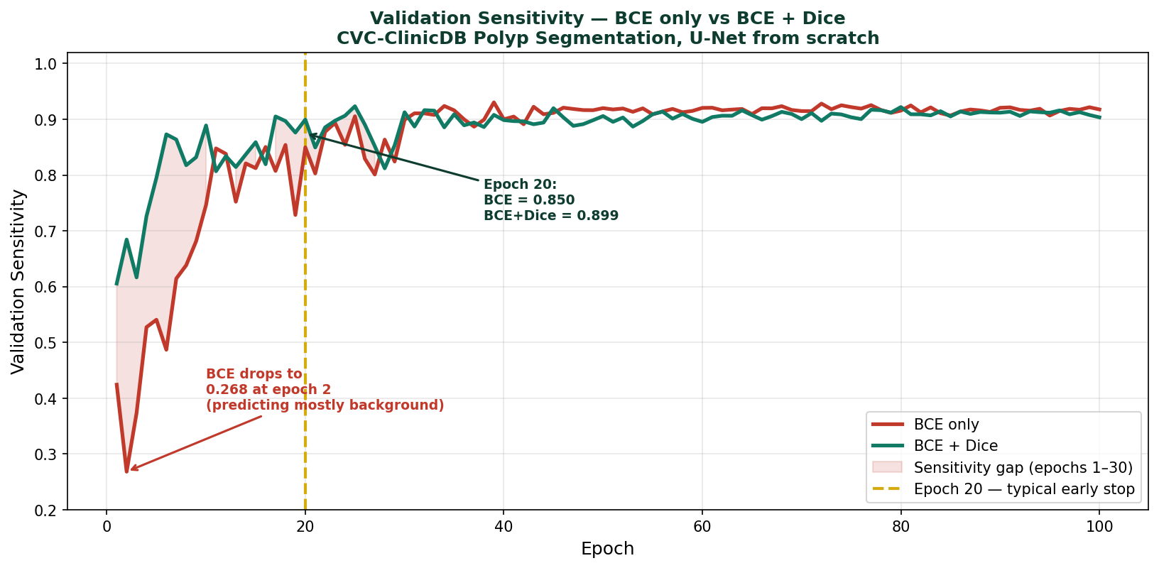
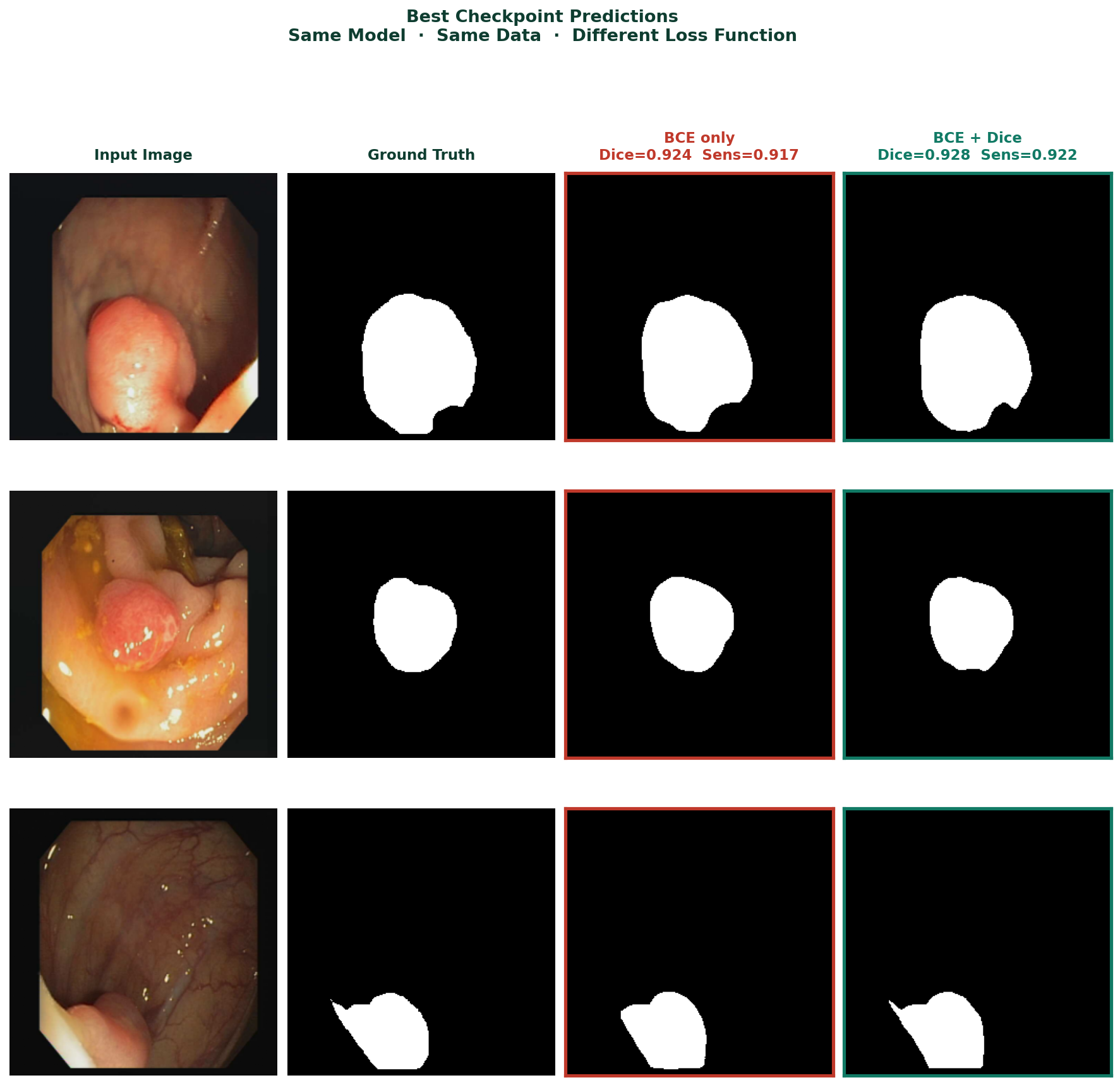
We will use CVC-ClinicDB polyp segmentation as the practical example throughout, the same dataset and model used in Blog 1 of this series. The training results shown here come from the U-Net trained from scratch with BCE + Dice loss in that post. If you have not read Blog 1, you do not need to, but if your model is predicting only background, that post addresses it directly.


The Problem U-Net Was Designed to Solve

Before U-Net existed, the standard approach to segmentation was to take a classification network, something like VGG or AlexNet, and adapt it to produce pixel-level output instead of a single class label.

This sounds reasonable. Classification networks are good at recognising what is in an image. Surely that knowledge can be extended to recognise what is in each pixel.

The problem is what happens to spatial information inside a classification network.

A classification network progressively reduces the spatial dimensions of its feature maps through pooling and strided convolutions. A 256×256 input passes through five downsampling stages and arrives at the bottleneck as an 8×8 feature map. The network then applies a global pooling operation and produces a single class prediction.

At that 8×8 stage, each position in the feature map corresponds to a 32×32 region of the original image. The model knows that something is present somewhere in that region. It does not know where exactly within the region.

For classification, that is fine. For segmentation, where you need to know the exact boundary of a polyp at pixel level, that spatial uncertainty is fatal.

Downsampling builds understanding. It destroys location. Segmentation needs both. That tension is the problem U-Net solves.

The Encoder: Building Understanding by Destroying Location

Encoder pathway showing spatial resolution decreasing and channels increasing

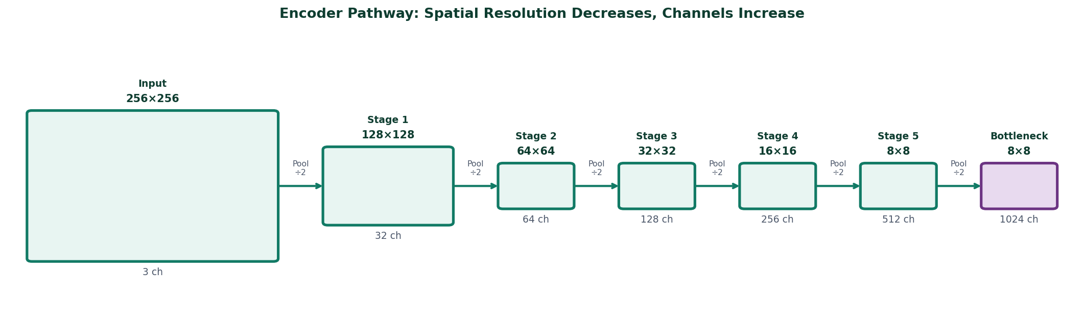
Figure 1 — The encoder pathway. A 256×256 input passes through five downsampling stages, arriving at the bottleneck as an 8×8 feature map with 1024 channels. Spatial resolution shrinks at each stage while channel depth grows, the network trades location precision for semantic understanding.

The encoder is the left half of U-Net. It applies two convolutional layers at each stage, followed by a max-pooling operation that halves the spatial dimensions before the next stage.

For a 256×256 input image, the five-stage encoder used in our CVC-ClinicDB model produces feature maps at the following resolutions:

Encoder Stage Feature Map Size Channels Receptive Field
Input256 × 25631 pixel
Stage 1 output256 × 25632~3 × 3 region
Stage 2 output128 × 12864~6 × 6 region
Stage 3 output64 × 64128~12 × 12 region
Stage 4 output32 × 32256~24 × 24 region
Stage 5 output16 × 16512~32 × 32 region
Bottleneck8 × 81024~64 × 64 region

Notice two things happening simultaneously. The spatial dimensions shrink, from 256×256 to 8×8, while the channel count grows, from 3 to 1024. The network is trading spatial resolution for representational depth. At the bottleneck, each of the 8×8 positions carries a rich 1024-dimensional description of a large region of the original image. It knows what is there. It has lost the fine-grained where.

This is by design, not by accident. The large receptive field at the bottleneck is what allows the network to understand global context, whether the overall image looks like it contains a large central polyp, or scattered small ones, or nothing unusual at all.


The Decoder: Trying to Recover What Was Lost

The decoder is the right half of U-Net. Its job is to take the bottleneck feature map, rich in semantic content but poor in spatial detail and progressively restore spatial resolution until the output matches the original image dimensions.

It does this through transposed convolution operations that reverse the encoder's pooling. At each stage, the feature map is spatially enlarged by a factor of two, and a pair of convolutional layers refines the upsampled features.

But here is the fundamental problem with a decoder operating alone.

Upsampling is not the inverse of downsampling. When max-pooling reduces a region to a single value, it retains the maximum and discards everything else. No upsampling operation can recover what was discarded. The decoder can produce a spatially large output, but that output will be blurry and imprecise at boundaries because the precise boundary information was lost during encoding and cannot be reconstructed from the bottleneck alone.

Analogy Imagine taking a high-resolution photograph, shrinking it to thumbnail size, and then enlarging it back to the original dimensions. The enlarged image has the right overall composition, you can see where the subject is, roughly what shape it has. But the fine detail, sharp edges, precise boundaries, is gone. No enlargement algorithm can invent detail that was not preserved.

This is exactly the problem that forced the skip connection into existence.


Skip Connections: The Actual Innovation

Skip connection diagram showing encoder stages connected directly to matching decoder stages

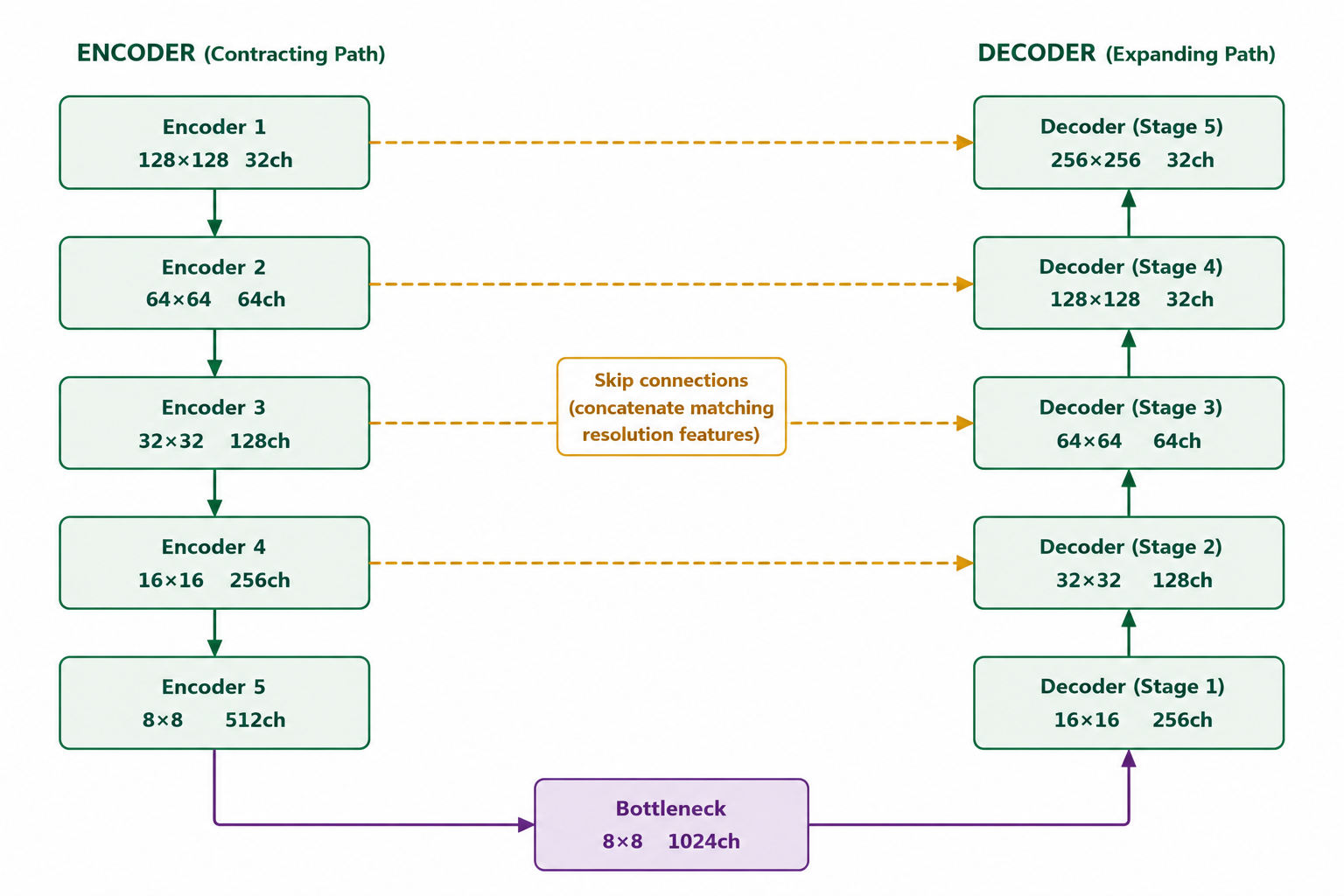
Figure 2 — Skip connections in U-Net. Each encoder stage passes its feature map directly to the corresponding decoder stage at the same spatial resolution. Encoder 1 (128×128) connects to Decoder 5 (128×128), Encoder 2 (64×64) to Decoder 4 (64×64), and so on. The bottleneck feeds into Decoder 1 (8×8), the first decoder stage. Decoder stages then upsample progressively toward the final output.

The skip connection is U-Net's defining contribution. Rather than requiring the decoder to reconstruct fine spatial detail from the bottleneck alone, it gives the decoder direct access to the encoder's feature maps at each spatial scale, before those maps were downsampled.

At each decoder stage, two sources of information are concatenated:

  • The upsampled feature map from the previous decoder stage, semantically rich, spatially coarse
  • The encoder feature map from the corresponding spatial scale, spatially precise, semantically shallow

The convolutional layers that follow the concatenation learn to integrate these two sources. The semantic information from the decoder path tells the network what the region is. The spatial information from the encoder path tells it exactly where the boundary is.

This is why U-Net produces sharp, precise segmentation boundaries when a decoder-only architecture produces blurry ones. The boundary precision does not come from clever upsampling. It comes from having direct access to the original encoder features that contained that precision before it was lost to downsampling.

Why Concatenation and Not Addition

Skip connections in U-Net use concatenation, the encoder and decoder feature maps are stacked along the channel dimension, doubling the channel count before the next convolution. ResNets use addition instead. The choice matters.

Addition requires the two tensors to have the same meaning for the operation to make sense, you are combining them into a single representation. Concatenation preserves both representations independently and lets the following convolution learn how to use each one. For segmentation, where the encoder and decoder features carry fundamentally different types of information, spatial precision vs semantic depth, concatenation is the right choice.


The Complete Architecture

Complete U-Net architecture with encoder, bottleneck, decoder and skip connections

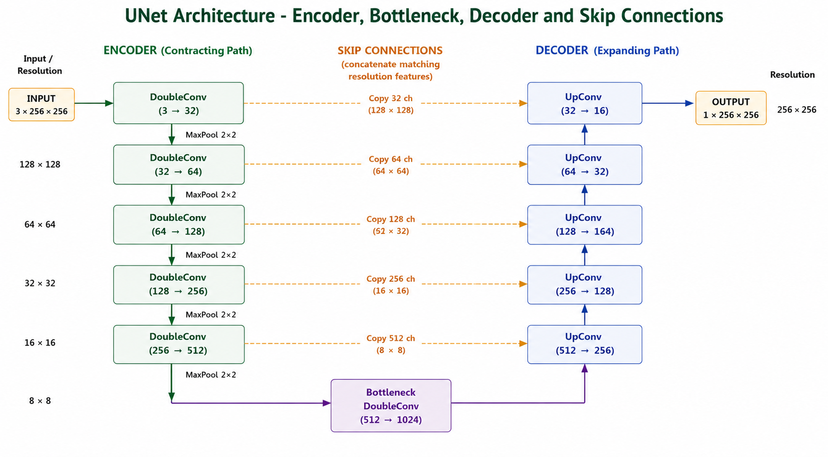
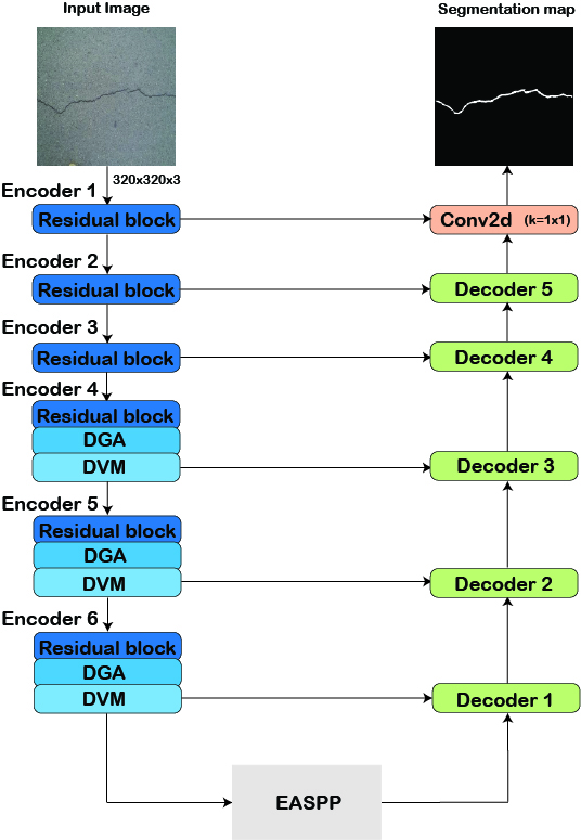
Figure 3 — Complete U-Net architecture as used in the CVC-ClinicDB polyp segmentation experiment. Five encoder stages compress a 256×256 input down to 8×8 at the bottleneck. Five decoder stages restore spatial resolution back to 256×256. Dashed amber arrows show the five skip connections transferring encoder feature maps directly to matching decoder stages. The 1×1 conv with sigmoid at the top of the decoder produces the final binary segmentation mask at full input resolution.

The complete U-Net has a symmetric structure, five encoder stages on the left, a bottleneck at the bottom, five decoder stages on the right, with skip connections bridging each encoder-decoder pair at the same spatial resolution.

The U shape is not an accident of diagram layout. It is a direct consequence of the architecture's function: compress spatial information as you go down, expand it as you go up, and maintain direct connections between the corresponding levels on each side.

📖 Segmentation Book 1 covers the U-Net architecture in full mathematical detail, including the precise equations for each operation, the role of batch normalization, and the design rationale behind the channel progression at each stage. Explore Segmentation Books

Training U-Net on CVC-ClinicDB — What It Actually Looks Like

The model used throughout this post is a U-Net trained from scratch on the CVC-ClinicDB colonoscopy polyp dataset. The channel widths follow the pattern [32, 64, 128, 256, 512] across the five encoder stages, with a 1024-channel bottleneck. The loss function is BCE + Dice combined, which was shown in Blog 1 to produce reliable foreground detection from the first epochs.

class DoubleConv(nn.Module):
    def __init__(self, in_channels, out_channels):
        super().__init__()
        self.conv = nn.Sequential(
            nn.Conv2d(in_channels, out_channels,
                      kernel_size=3, padding=1,
                      bias=False),
            nn.BatchNorm2d(out_channels),
            nn.ReLU(inplace=True),
            nn.Conv2d(out_channels, out_channels,
                      kernel_size=3, padding=1,
                      bias=False),
            nn.BatchNorm2d(out_channels),
            nn.ReLU(inplace=True),
        )

    def forward(self, x):
        return self.conv(x)


class UNET(nn.Module):
    def __init__(self, num_classes=1,
                 input_channels=3, **kwargs):
        super().__init__()
        nb_filter = [32, 64, 128, 256, 512]
        self.pool = nn.MaxPool2d(2, 2)

        # Encoder
        self.conv0_0 = DoubleConv(input_channels, nb_filter[0])
        self.conv1_0 = DoubleConv(nb_filter[0],   nb_filter[1])
        self.conv2_0 = DoubleConv(nb_filter[1],   nb_filter[2])
        self.conv3_0 = DoubleConv(nb_filter[2],   nb_filter[3])
        self.conv4_0 = DoubleConv(nb_filter[3],   nb_filter[4])

        # Bottleneck
        self.bottleneck = DoubleConv(nb_filter[4], nb_filter[4] * 2)

        # Decoder
        self.upconv4 = nn.ConvTranspose2d(nb_filter[4] * 2, nb_filter[4], 2, 2)
        self.conv4_1 = DoubleConv(nb_filter[4] * 2, nb_filter[4])

        self.upconv3 = nn.ConvTranspose2d(nb_filter[4], nb_filter[3], 2, 2)
        self.conv3_2 = DoubleConv(nb_filter[3] * 2, nb_filter[3])

        self.upconv2 = nn.ConvTranspose2d(nb_filter[3], nb_filter[2], 2, 2)
        self.conv2_3 = DoubleConv(nb_filter[2] * 2, nb_filter[2])

        self.upconv1 = nn.ConvTranspose2d(nb_filter[2], nb_filter[1], 2, 2)
        self.conv1_4 = DoubleConv(nb_filter[1] * 2, nb_filter[1])

        self.upconv0 = nn.ConvTranspose2d(nb_filter[1], nb_filter[0], 2, 2)
        self.conv0_5 = DoubleConv(nb_filter[0] * 2, nb_filter[0])

        self.final = nn.Conv2d(nb_filter[0], num_classes, kernel_size=1)

    def forward(self, x):
        x0_0 = self.conv0_0(x)
        x1_0 = self.conv1_0(self.pool(x0_0))
        x2_0 = self.conv2_0(self.pool(x1_0))
        x3_0 = self.conv3_0(self.pool(x2_0))
        x4_0 = self.conv4_0(self.pool(x3_0))
        x5_0 = self.bottleneck(self.pool(x4_0))

        x4_1 = self.conv4_1(
            torch.cat([self.upconv4(x5_0), x4_0], dim=1))
        x3_2 = self.conv3_2(
            torch.cat([self.upconv3(x4_1), x3_0], dim=1))
        x2_3 = self.conv2_3(
            torch.cat([self.upconv2(x3_2), x2_0], dim=1))
        x1_4 = self.conv1_4(
            torch.cat([self.upconv1(x2_3), x1_0], dim=1))
        x0_5 = self.conv0_5(
            torch.cat([self.upconv0(x1_4), x0_0], dim=1))

        return torch.sigmoid(self.final(x0_5))


def criterion(pred, mask):
    return bce_loss(pred, mask) + dice_loss(pred, mask)

What Predictions Look Like at Different Training Stages

U-Net prediction progression at epochs 1, 20, 50 and 100

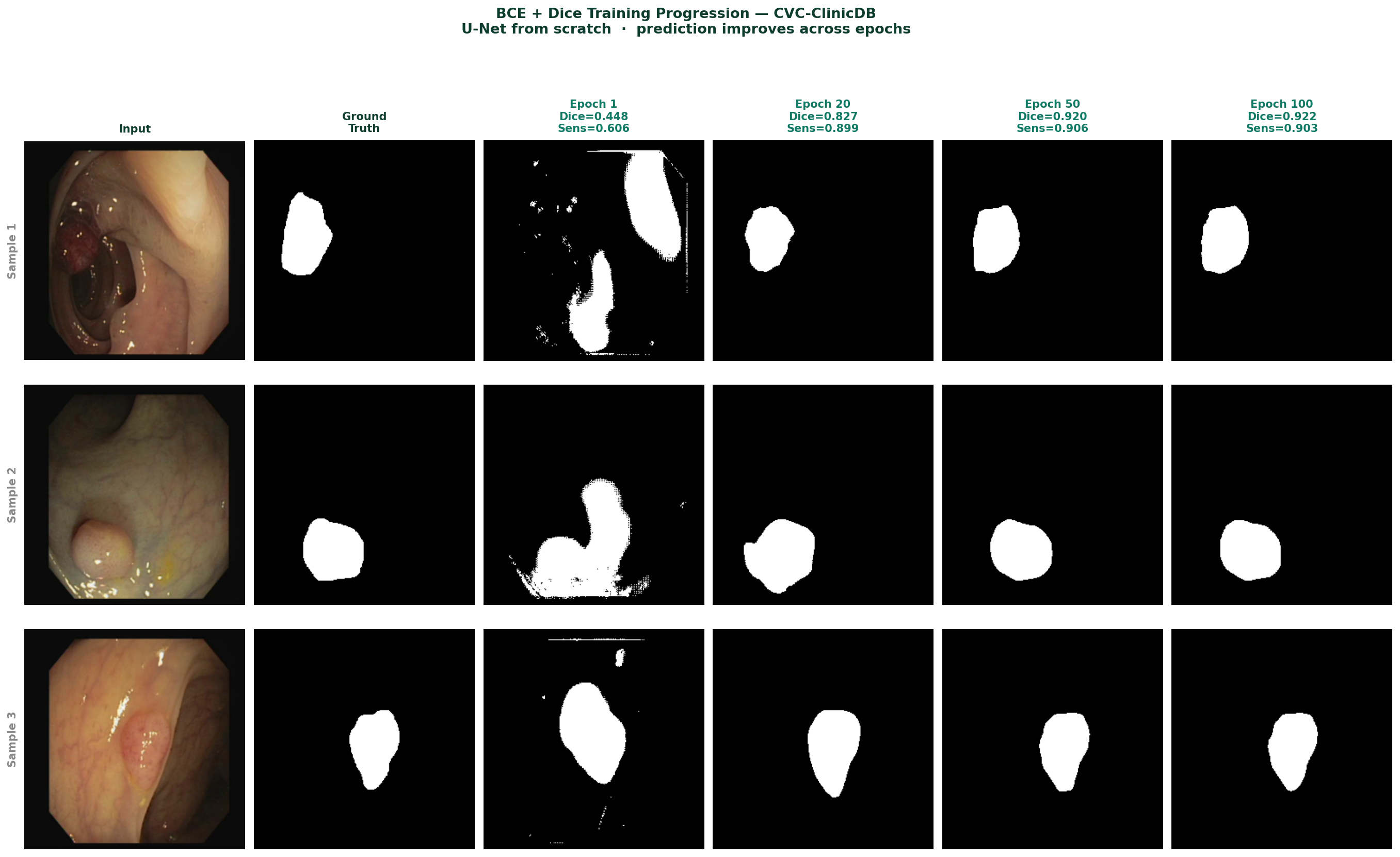
Figure 4 — U-Net predictions on CVC-ClinicDB test images at epochs 1, 20, 50, and 100. Epoch 1: rough initial detection with noisy boundaries and false positives. Epoch 20: recognisable polyp shapes with improved boundaries, Dice 0.827. Epoch 50: clean segmentation, Dice 0.920. Epoch 100: precise boundaries closely matching ground truth, Dice 0.922.

The progression of predictions across epochs reflects what the model is learning in sequence. It learns the global presence of a polyp before it learns its extent, and it learns approximate extent before it learns precise boundaries. The skip connections are what enable the final stage, precise boundaries require the spatial detail that the encoder preserved, and that detail only becomes useful to the decoder after it has learned the semantic context from the bottleneck.


Training Curves

U-Net training curves showing IoU, Dice, Sensitivity and Specificity over 100 epochs

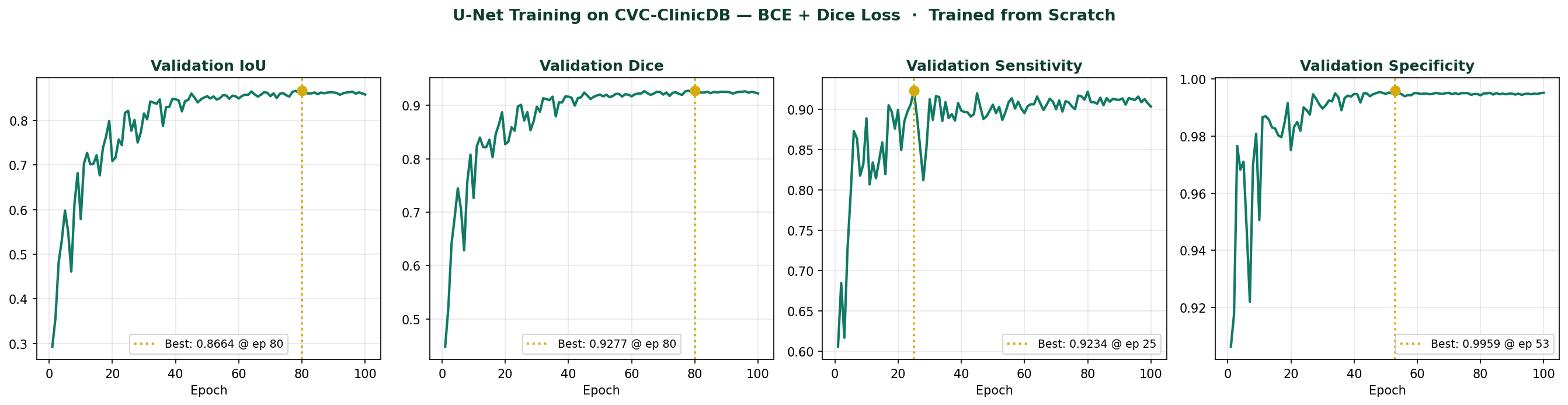
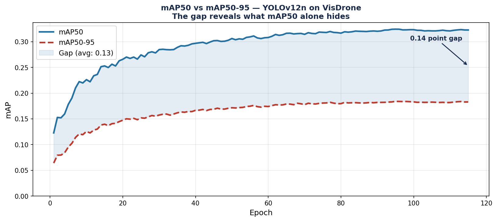
Figure 5 — Validation metrics over 100 training epochs. IoU and Dice converge steadily, reaching best values of 0.8664 and 0.9277 respectively at epoch 80. Sensitivity peaks at 0.9234 at epoch 25. Specificity reaches 0.9959 at epoch 53. All metrics plateau after epoch 60, indicating full convergence.

The training curves confirm the pattern established in Blog 1. BCE + Dice produces reliable sensitivity from the first epochs, the model finds polyps early and refines boundary precision over subsequent epochs. The IoU and Dice curves show steady improvement without collapse, which is the signature of a well-functioning loss function on an imbalanced dataset.


What U-Net Does Not Do Well

Understanding the architecture's limitations is as important as understanding its strengths.

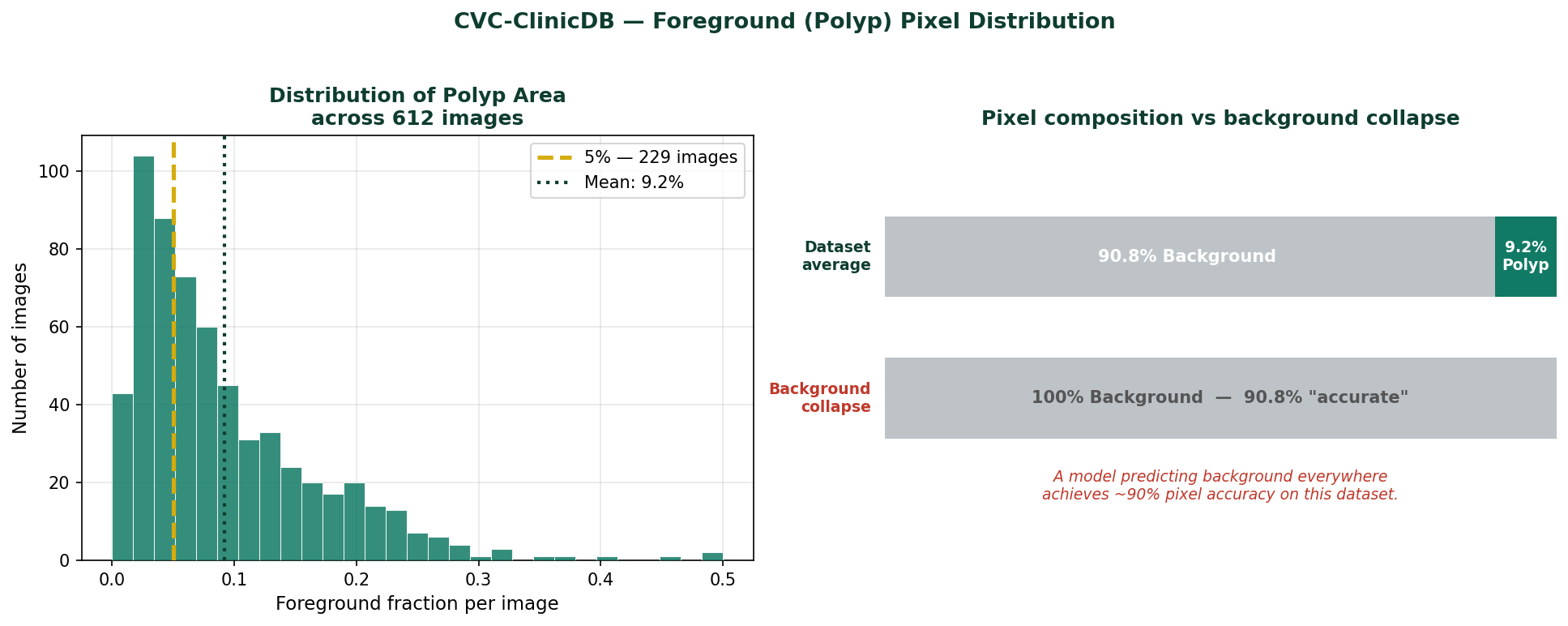
Very small objects. When a polyp occupies only 1 to 2% of the image area, it may be represented by just a handful of pixels at the bottleneck. The global context is dominated by the surrounding healthy tissue. The model has very little signal to work with for objects this small. Higher input resolution and specialized loss functions help, but the fundamental constraint is architectural.

Computational cost at high resolution. The five-stage U-Net with channel widths [32, 64, 128, 256, 512] has approximately 7 million parameters. At 512×512 input, a batch of eight images requires substantial GPU memory. Scaling to higher resolutions quickly hits hardware limits.

Multiscale feature capture at the bottleneck. The standard U-Net bottleneck applies the same double-convolution block used throughout the encoder. It has no dedicated mechanism for capturing contextual information at multiple scales simultaneously, a limitation that more recent architectures address explicitly through modules like ASPP or dilated convolution pyramids.

U-Net's skip connections solve the spatial precision problem elegantly. The limitations that remain, small object detection, computational cost, and multiscale context at the bottleneck, are the problems that drive architecture research beyond the baseline.
📖 Segmentation Book 1 covers all three limitations in detail, with practical strategies for each. The following two books in the series address the architectural solutions that have emerged from research on these specific failure modes. Explore Segmentation Books

Selected implementations, supporting utilities, and companion resources related to this article are available through the Blog 3 Companion Resources page .

Companion Resources Included

  • U-Net architecture implementation
  • DoubleConv block reference
  • U-Net training configuration
  • Skip connection logic reference
  • Training curve plotting utility
  • Architecture figure notes

The One Thing to Remember

U-Net works because it gives the decoder direct access to the spatial detail that the encoder preserved before discarding it through downsampling. The skip connections are not a regularization trick or an optimization convenience. They are the solution to a specific, fundamental problem, the irrecoverable loss of spatial information during encoding.

Every modern segmentation architecture that outperforms U-Net does so by addressing one of the limitations listed above, while keeping the core encoder-decoder-skip-connection structure intact. Understanding why U-Net is designed the way it is makes those improvements immediately comprehensible, because you can see exactly which problem each one is solving.


Training a segmentation model and running into issues this post does not cover?
Feel free to reach out through occulins.com/contact

Tags: U-Net Semantic Segmentation Skip Connections Encoder Decoder CVC-ClinicDB Polyp Segmentation Medical Imaging Deep Learning Architecture
Resources

Blog 3 Companion Resources.

Supporting assets for the article: U-Net Explained Clearly, architecture logic, skip connections, encoder-decoder structure, and selected visualization utilities.

U-Net Implementation

Reference U-Net implementation used across the related segmentation articles.

Previously Added

DoubleConv Block

Reusable two-layer convolution block used throughout the U-Net encoder, bottleneck, and decoder stages.

Previously Added

U-Net Configuration

Architecture setup and training configuration used during the CVC-ClinicDB segmentation experiments.

Previously Added

Skip Connection Logic

Minimal reference showing how encoder features are concatenated with decoder features at matching spatial scales.

Architecture Logic

Training Curve Plotting

Selected plotting utility for visualizing validation Dice and IoU across training epochs.

Visualization

Figure Notes

Short notes describing how the explanatory U-Net figures were structured for clarity and progressive understanding.

Figure Guide

Resource Notes

Selected resources are designed to support experimentation and practical understanding through focused implementations, utilities, and companion materials accompanying each article.

Return to Blog 3

Resources

Skip Connection Logic.

Minimal example showing how encoder features are fused with decoder features at matching spatial resolutions.


decoder_feature = upsample(

    decoder_feature

)

fusion = torch.cat(

    [

        encoder_feature,

        decoder_feature

    ],

    dim=1

)
Resources

Training Curve Plotting.

Utility for visualizing validation metrics during training.


plt.plot(

epochs,

history['val_dice'],

label='Dice'

)

plt.plot(

epochs,

history['val_iou'],

label='IoU'

)

plt.xlabel(

'Epoch'

)

plt.ylabel(

'Metric'

)

plt.legend()

plt.grid(True)

plt.show()
Resources

Figure Notes.

Design philosophy behind the explanatory architecture figures.

Architecture figures were intentionally designed to progressively explain encoder behavior, skip connections, feature hierarchy, and information flow while maintaining visual consistency across diagrams.

Visual complexity was reduced by emphasizing resolution transitions, channel growth, and feature propagation instead of implementation-level detail.

Figures prioritize conceptual understanding and visual clarity rather than framework-specific implementation details.

Return to Blog 3 Resources

Debugging & Failure Analysis

Common Mistakes in Object Detection Training
That Kill Performance

By Dr. Ali Khan  |  Occulins


Object detection training failures share an uncomfortable characteristic: they are often invisible until you look in the right place.

A model can train for a hundred epochs, produce a respectable mAP number, and still be fundamentally broken, predicting the wrong classes, failing on the objects that matter most, or performing well only because the validation set leaked into training. The loss curves look fine. The metrics look acceptable. The predictions on casual inspection look plausible.

After years of working on detection problems across aerial imagery, medical imaging, and industrial inspection, I have seen the same mistakes appear repeatedly, not because the people making them are careless, but because the mistakes are genuinely subtle and the feedback signals that would reveal them are easy to overlook.

This post covers four of them. Each one has a specific symptom pattern that tells you it is present, and a specific fix that resolves it. None of them require changing your architecture or your hardware. All of them require paying closer attention to things you may currently be skipping.


1
Wrong or Inconsistent Annotations

This is the most common root cause of poor detection performance, and the one most rarely investigated because it requires looking at data rather than adjusting training parameters.

Annotation errors come in several forms, and they have different effects on training. Understanding which type you have determines what to do about it.

Tight vs Loose Bounding Boxes

Different annotators, or even the same annotator on different days, draw bounding boxes with different tightness. One person draws the box flush to the visible object edges. Another adds a few pixels of margin. A third includes part of the background context.

When a model is trained on this mixed data, it learns an inconsistent definition of where an object ends and background begins. During inference, predicted boxes are evaluated against ground truth boxes using IoU. If your ground truth boxes are inconsistently sized, your IoU measurements are measuring annotator inconsistency as much as model performance.

Three annotation styles on the same object

Figure 1 — Three annotation styles on the same object: tight (flush to visible edges), loose (2–5px margin), and inconsistent (partial background included). A training set mixing all three styles produces a model that learns no consistent boundary definition.

Inconsistent Class Definitions

This is harder to detect and more damaging than box tightness variation. It happens when the same visual object is labelled differently depending on context, annotator, or a class definition that was never written down precisely.

Common examples: a partially occluded car labelled as "car" in one image and ignored in another. A person on a bicycle labelled as "person" in some images and "cyclist" in others when cyclist is not a defined class. A van labelled as "car" by one annotator and "truck" by another.

The symptom in training is a class loss that decreases slowly or plateaus early, and a confusion matrix where two specific classes consistently swap with each other. If you see that pattern, look at the annotations for those two classes directly.

The Silent Problem: Missing Labels

In YOLO format, an image with no objects should have an empty label file. An image with objects but a missing label file is treated as a negative example — the model is taught that the objects in that image are background. This is one of the most damaging annotation errors because it actively teaches the model wrong information, not just inconsistent information.

Verify this before training:

import os

img_dir   = 'dataset/images/train'
label_dir = 'dataset/labels/train'

missing = []
for img_file in os.listdir(img_dir):
    stem       = os.path.splitext(img_file)[0]
    label_file = os.path.join(label_dir, stem + '.txt')
    if not os.path.exists(label_file):
        missing.append(img_file)

print(f"Images with no label file: {len(missing)}")
for f in missing[:10]:
    print(f"  {f}")

If this returns more than zero for a dataset that should have objects in every image, the missing label files are training your model to ignore those objects.

Symptom pattern Class loss plateaus early. Confusion matrix shows two classes swapping frequently. Model misses objects that are clearly visible in validation images. mAP is lower than expected given the apparent quality of your images.
Fix Define class boundaries in writing before annotating, not after. Spot-check 50 random image-label pairs visually before training. Run the missing label verification script above. If you find inconsistent annotations, correct them rather than hoping the model learns through them.
2
Augmentation That Hurts More Than It Helps

Data augmentation is universally recommended, and for good reason, it is one of the most effective tools for improving generalization on limited datasets. But augmentation is not a dial you turn up for better performance. The wrong augmentation strategy can actively damage your model, and the damage is difficult to diagnose because the training metrics often look fine while it is happening.

Augmentation That Destroys Small Objects

The most common augmentation mistake in detection is applying aggressive random cropping or zooming-out on datasets where objects are small relative to the image. When you randomly crop 40% of a 640×640 image, a pedestrian that was 20 pixels tall may disappear entirely, but its label file still says a pedestrian is present. The model is being trained on images where the labelled object is no longer visible.

For aerial datasets with small objects, the safe augmentation operations are flipping, rotation, and mild color jitter. Heavy cropping, large-scale mosaic augmentation with significant zoom-out, and perspective transforms that shrink objects further are all candidates for removal.

Color Augmentation on Domain-Specific Imagery

Aggressive color jitter is appropriate for natural photography where color balance varies widely between cameras and lighting conditions. It is not appropriate for datasets acquired under controlled conditions, certain medical imaging formats, thermal imagery, or nighttime surveillance footage where color characteristics are fixed by the acquisition protocol.

If your deployment images will always look roughly the same in terms of color and exposure, training on aggressively color-jittered images teaches the model to be robust to variation it will never encounter, while reducing its precision on the actual color characteristics of your domain.

Mosaic Augmentation and Dense Small Objects

YOLO's mosaic augmentation combines four images into one training sample. For most datasets this improves performance by exposing the model to more objects per forward pass. For datasets with very dense small objects, aerial imagery, crowd detection, microscopy, mosaic can produce images where object density exceeds anything in the real deployment distribution. The model learns to expect densities it will never see, which affects both detection thresholds and confidence calibration.

Augmentation is not universally beneficial Every augmentation operation should be evaluated on your specific dataset. The default augmentation settings in any framework were tuned on benchmark datasets that may not resemble yours. Check whether disabling or reducing specific augmentations improves your validation mAP, not just your training stability.
Symptom pattern Model detects objects of normal size but consistently misses small ones. Confidence scores are poorly calibrated, very high or very low, with few in the middle range. Disabling augmentation temporarily and retraining produces higher validation mAP than with augmentation enabled.
Fix Start with minimal augmentation, horizontal flip and mild color jitter only. Add operations one at a time and measure their effect on validation mAP. If an augmentation does not improve validation performance after 20 epochs, remove it. For small-object datasets, be especially conservative with any operation that reduces object size.
📖 Detection Book 2 covers domain-specific augmentation strategy in detail, including which operations help and which hurt for aerial, medical, and industrial detection tasks. Explore Detection Books
3
Poor Evaluation — The Metric You Report Is Not What You Think

This mistake does not affect how your model trains. It affects whether you know what your model can actually do. Reporting the wrong metric, or computing the right metric on the wrong data, produces numbers that look good while hiding real failures.

mAP50 vs mAP50-95: A Gap That Changes Everything

mAP50 evaluates detection at a single IoU threshold of 0.5. A predicted box that overlaps the ground truth by 50% counts as a correct detection. This is a lenient standard, a box that covers the correct general region but is significantly larger or smaller than the actual object still passes.

mAP50-95 averages detection performance across IoU thresholds from 0.5 to 0.95 in steps of 0.05. At IoU 0.75, a predicted box needs to overlap 75% with the ground truth to count. At IoU 0.95, the box needs to be almost pixel-perfect.

For applications where precise bounding box location matters, measuring object size, feeding detections into a tracking system, or using boxes to guide downstream processing — mAP50-95 is the metric that tells you whether your model is accurate enough. mAP50 can look 15 to 25 points higher than mAP50-95 on the same model.

mAP50 vs mAP50-95 across training epochs

Figure 2 — mAP50 vs mAP50-95 across training epochs for YOLOv12n on VisDrone. mAP50 reaches 0.325 while mAP50-95 plateaus at 0.185, a gap that reflects the model's ability to find objects in the right location but not localise them precisely. The shaded region between the two curves is what mAP50 alone hides. Always report both metrics.

Evaluating on Training Data

This sounds too basic to mention. It is not. It happens more often than it should, in two forms.

The first form is accidental: the validation data path in the YAML file points to the training directory due to a typo or copy-paste error. The model evaluates on data it has already memorised. Validation mAP is inflated by 10 to 30 points depending on how long the model has trained.

The second form is subtle: the validation split was created by random sampling at the image level from a dataset where multiple images came from the same video sequence or the same scene. Frames from the same scene look nearly identical. A model that has seen other frames from the same scene during training will perform well on the validation frames, not because it generalizes, but because it has effectively memorised the scene.

import yaml

with open('dataset.yaml') as f:
    cfg = yaml.safe_load(f)

print("Train path:", cfg.get('train'))
print("Val path:",   cfg.get('val'))

assert cfg['train'] != cfg['val'], \
    "Train and val paths are identical — check your YAML"

Ignoring Per-Class Performance

Mean Average Precision averages across all classes. A model that achieves 0.72 mAP on a ten-class dataset may be achieving 0.90 on five common classes and 0.50 on five rare ones. If the rare classes are the ones that matter in your application, the aggregate number is hiding a failure.

Always look at per-class AP alongside the mean. In Ultralytics, the per-class results are printed at the end of validation. Read them, not just the summary line.

Symptom pattern Validation mAP looks strong but model fails visually on many predictions. Performance in deployment is significantly worse than validation numbers suggested. Per-class AP shows large variance across classes.
Fix Always report both mAP50 and mAP50-95. Verify your train and val paths are different before every training run. Split datasets with sequential or scene-grouped images at the scene level, not the image level. Read per-class AP after every evaluation.
📖 Detection Book 1 covers evaluation metrics in depth, including when each metric is appropriate, how to interpret per-class results, and what the numbers actually tell you about deployment readiness. Explore Detection Books
4
Overfitting — And Why It Is Harder to Spot Than You Think

Overfitting in detection is not always the obvious case where training loss goes to zero and validation loss spikes. In practice it is often subtler, a model that performs well on the validation set but fails on genuinely new data from a slightly different source.

The Classic Pattern

The textbook version of overfitting is easy to diagnose from the loss curves: training loss decreases steadily while validation loss plateaus or begins to rise. If you see this pattern, the model is memorising the training set rather than learning generalizable features.

Healthy training vs overfitting loss curves

Figure 3 — Left: healthy training, training and validation loss decrease together and converge. Right: overfitting, training loss continues decreasing while validation loss plateaus and begins rising. The gold dotted line marks the best checkpoint, the model should be saved here, not at the end of training.

The Hidden Pattern: Dataset Overfitting

The more dangerous form of overfitting does not show up in your loss curves at all. The model generalises well to your validation set, but your validation set is not representative of deployment conditions.

This happens when training and validation data come from the same source, same time period, same camera, or same geographic location, while deployment data comes from a different source. The model has learned the specific visual characteristics of your dataset, a particular camera's color profile, the typical lighting conditions of a specific location, the image quality of a specific acquisition protocol, rather than the underlying object appearance.

The only way to detect this is to evaluate on truly independent test data from a different source than your training data. If performance drops significantly on that data, your model has overfit to your dataset distribution.

How to Actually Fix Overfitting

The standard advice, more data, more dropout, stronger augmentation, is correct but incomplete. The more important question is why the model is overfitting, because the answer determines the right fix.

  • Model is too large for the dataset: switch to a smaller model variant before adding regularization. A nano model on a 500-image dataset overfits less than a large model with dropout.
  • Dataset lacks diversity: augmentation helps but is not a substitute for genuinely diverse data. If all your training images come from one camera at one location, no augmentation strategy will teach the model to handle a different camera at a different location.
  • Training too long: use early stopping based on validation mAP. Save the best checkpoint, not the final one. The final epoch is almost never the best model.
Symptom pattern Validation mAP is strong but performance drops noticeably when tested on images from a different source, time period, or camera. Training loss is significantly lower than validation loss. Per-class performance is strong on common classes and weak on rare ones.
Fix Use early stopping. Save the best checkpoint based on validation mAP, not the final epoch. Evaluate on a held-out test set from a different source than your training data. Start with the smallest model that achieves acceptable performance rather than the largest.
📖 Detection Book 2 covers domain shift and dataset diversity in depth, including how to evaluate whether your model will hold up in deployment and what to do when it does not. Explore Detection Books

The Mistake That Ties All of Them Together

Each of the four mistakes above has something in common: they are all invisible if you only look at your final training metrics.

Wrong annotations produce acceptable loss curves. Bad augmentation produces acceptable training stability. Poor evaluation produces numbers that look fine. Overfitting produces good validation metrics right up until you test on new data.

The habit that prevents all four is simple, and almost nobody does it consistently: look at your actual data and your actual predictions at every stage of the pipeline, not just the numbers that summarise them.

Open five random training images and verify the labels visually before training starts. Save prediction images every ten epochs during training and look at them. Read per-class AP after every evaluation. Test on data from a different source before declaring success. These four habits cost fifteen minutes per training run and prevent the majority of detection failures.

Selected implementations, supporting utilities, and companion resources related to this article are available through the Blog 4 Companion Resources page .

Companion Resources Included

  • Missing label verification utility
  • Annotation inspection checklist
  • Train / validation path verification utility
  • mAP interpretation reference notes
  • Overfitting diagnostics guide
  • Pre-deployment evaluation checklist

Quick Reference

Mistake Symptom Fix
Wrong annotationsClass loss plateaus, classes swap in confusion matrixDefine classes in writing, spot-check 50 pairs, verify no missing labels
Bad augmentationSmall objects missed, poor confidence calibrationStart minimal, add one operation at a time, measure each addition
Poor evaluationStrong metrics, weak real-world performanceReport mAP50 and mAP50-95, verify val path, split at scene level
OverfittingVal loss rises, deployment performance dropsEarly stopping, smallest sufficient model, independent test data

These mistakes are not signs of inexperience, they appear in research projects and production systems alike. What separates teams that catch them quickly from those that spend weeks on the wrong problem is the habit of looking at data and predictions directly, rather than trusting that metrics alone will surface the issue.

The metrics will not surface the issue. They will hide it.


Working on a detection project and running into performance problems that this post does not fully resolve?
Feel free to reach out through occulins.com/contact

Tags: Object Detection Training Mistakes Annotations Data Augmentation Overfitting mAP Evaluation Deep Learning YOLOv12
Resources

Blog 4 Companion Resources.

Supporting assets for debugging object detection training failures, dataset verification, evaluation sanity checks, and failure analysis workflows.

Missing Label Verification

Utility for identifying training images without corresponding annotation files.

Dataset Verification

Annotation Inspection Workflow

Simple workflow for visually validating image-label pairs before training begins.

Quality Control

Train / Validation Verification

Utility for checking dataset splits and preventing train-validation leakage.

Configuration Check

mAP Interpretation

Reference helper for understanding the difference between mAP50 and mAP50-95.

Evaluation

Overfitting Diagnostics

Guidelines for identifying memorization and poor generalization behavior.

Failure Analysis

Evaluation Checklist

Pre-deployment sanity checklist before trusting validation metrics.

Checklist

Resource Notes

Selected resources are designed to support experimentation and practical understanding through focused implementations, utilities, and companion materials accompanying each article.

Return to Blog 4

Resources

Missing Label Verification.

Check whether each training image has a matching YOLO annotation file.

import os

image_dir = "images/train"
label_dir = "labels/train"

images = {
    os.path.splitext(f)[0]
    for f in os.listdir(image_dir)
}

labels = {
    os.path.splitext(f)[0]
    for f in os.listdir(label_dir)
}

missing = images - labels

print(f"Missing labels: {len(missing)}")

for item in sorted(missing):
    print(item)
Resources

Annotation Inspection Workflow.

A practical checklist for visually validating image-label pairs before training.

  • Verify image-label alignment visually
  • Inspect bounding box placement
  • Check class assignments
  • Check empty labels
  • Inspect duplicate images
  • Check class imbalance
Resources

Train / Validation Verification.

Check dataset paths to avoid train-validation leakage.

import yaml

with open("dataset.yaml", "r") as f:
    cfg = yaml.safe_load(f)

print("Train path:", cfg["train"])
print("Validation path:", cfg["val"])

assert cfg["train"] != cfg["val"], \
    "Train and validation paths are identical. Check your YAML file."
Resources

mAP Interpretation.

Quick notes for interpreting mAP50 and mAP50-95 together.

High mAP50 with lower mAP50-95 often indicates localization weakness rather than complete detection failure.

Large gaps suggest predictions may detect objects correctly but produce poorly aligned bounding boxes.

Always inspect qualitative predictions and per-class AP instead of relying on one aggregate metric.

Resources

Overfitting Diagnostics.

Practical signs that a detector is memorizing instead of generalizing.

  • Training loss decreases while validation loss rises
  • Large train-validation metric gap
  • Performance drops on images from unseen sources
  • Validation metrics become unstable across epochs
  • Rare classes perform much worse than common classes
Resources

Evaluation Checklist.

Pre-deployment sanity checklist before trusting validation metrics.

  • Inspect prediction visualizations
  • Check per-class metrics
  • Review failure cases
  • Compare mAP50 and mAP50-95
  • Inspect false positives and false negatives
  • Verify train and validation paths
  • Validate deployment constraints